How to Use PRONE for the Evaluation of Normalization Methods on Spike-In Data

library(PRONE)

Spike-in Data Sets

PRONE also offers some additional functionalities for the evaluation of normalization techniques on spike-in data sets with a known ground truth. These functionalities will be delineated subsequently. Additionally, all functionalities detailed in the context of real-world data sets remain applicable to the SummarizedExperiment object associated with spike-in data sets.

The example spike-in data set is from (Cox et al. 2014). For the illustration of the package functionality, a smaller subset of the data consisting of 1500 proteins was used. For the complete data set, please refer to the original publication.

Load Data

Initially, the spike-in data set needs to be imported into a SummarizedExperiment container. In contrast to the real-world data sets, you need to specify the “spike_column”, “spike_value”, “spike_concentration”, and utilize the load_spike_data() function for this purpose.

Here, the “spike_column” denotes the column in the protein intensity data file encompassing information whether a proteins is classified as spike-in or background protein. The “spike_value” determines the value/identifier that is used to identify the spike-in proteins in the “spike_column”, and the “spike_concentration” identifies the column containing the concentration values of the spike-in proteins (in this case the different conditions that will be tested in DE analysis).

data_path <- readPRONE_example("Ecoli_human_MaxLFQ_protein_intensities.csv")
md_path <- readPRONE_example("Ecoli_human_MaxLFQ_metadata.csv")

data <- read.csv(data_path)
md <- read.csv(md_path)

# Check if some protein groups are mixed
mixed <- grepl("Homo sapiens.*Escherichia|Escherichia.*Homo sapiens", data$Fasta.headers)
data <- data[!mixed,]

data$Spiked <- rep("HUMAN", nrow(data))
data$Spiked[grepl("ECOLI", data$Fasta.headers)] <- "ECOLI"

se <- load_spike_data(data, md, spike_column = "Spiked", spike_value = "ECOLI", spike_concentration = "Concentration",protein_column = "Protein.IDs", gene_column = "Gene.names", ref_samples = NULL, batch_column = NULL, condition_column = "Condition", label_column = "Label")

Overview of the Data

To get an overview on the number of identified (non-NA) spike-in proteins per sample, you can use the plot_identified_spiked_proteins() function.

plot_identified_spiked_proteins(se)
#> Condition of SummarizedExperiment used!
#> Label of SummarizedExperiment used!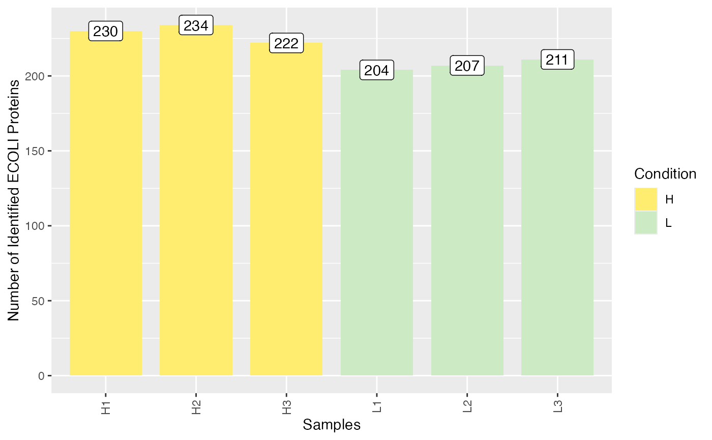

To compare the distributions of spike-in and human proteins in the different sample groups (here high-low), use the function plot_histogram_spiked(). Again, “condition = NULL” means that the condition specified by loading the data is used, but you can also specify any other column of the meta data.

plot_histogram_spiked(se, condition = NULL)
#> Condition of SummarizedExperiment used!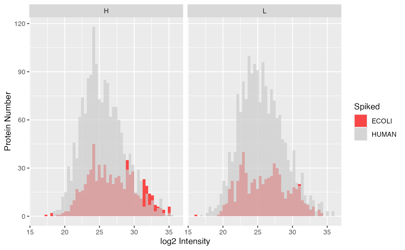

If you want to have a look at the amount of actual measure spike-in, you can use the plot_profiles_spiked() function. Moreover, you can analyze whether the intensities of the background proteins, here HUMAN proteins, are constant across the different spike-in concentrations.

plot_profiles_spiked(se, xlab = "Concentration")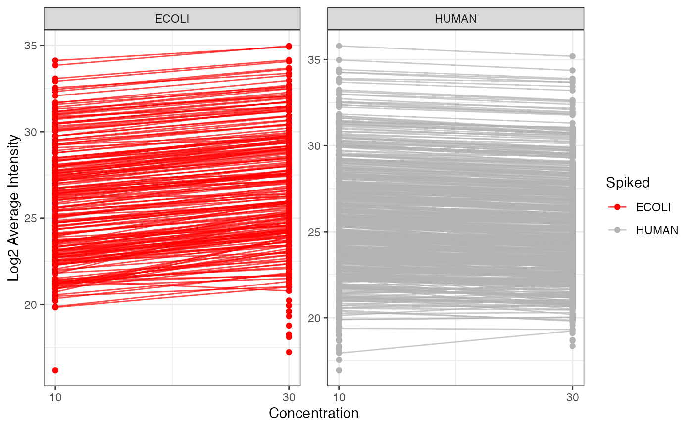

Preprocessing, Normalization, & Imputation

Given that the preprocessing (including filtering of proteins and samples), normalization, and imputation operations remain invariant for spike-in data sets compared to real-world data sets, the same methodologies can be employed across both types. In this context, normalization will only be demonstrated here as the performance of the methods will be evaluated in DE analysis, while detailed descriptions of the other functionalities are available in preceding sections.

se_norm <- normalize_se(se, c("Median", "Mean", "MAD", "LoessF"), combination_pattern = NULL)
#> Median completed.
#> Mean completed.
#> MAD completed.
#> LoessF completed.

Differential Expression Analysis

Due to the known spike-in concentrations, the normalization methods can be evaluated based on their ability to detect DE proteins. The DE analysis can be conducted using the same methodology as for real-world data sets. However, other visualization options are available and performance metrics can be calculated for spike-in data sets.

Run DE Analysis

First, you need to specify the comparisons you want to perform in DE analysis. For this, a special function was developed which helps to build the right comparison strings.

comparisons <- specify_comparisons(se_norm, condition = "Condition", sep = NULL, control = NULL)

Then you can run DE analysis:

de_res <- run_DE(se = se_norm, 
                     comparisons = comparisons,
                     ain = NULL, 
                     condition = NULL, 
                     DE_method = "limma", 
                     covariate = NULL, 
                     logFC = TRUE, 
                     logFC_up = 1, 
                     logFC_down = -1, 
                     p_adj = TRUE, 
                     alpha = 0.05, 
                     B = 100, 
                     K = 500)
#> Condition of SummarizedExperiment used!
#> All assays of the SummarizedExperiment will be used.
#> DE Analysis will not be performed on raw data.
#> log2: DE analysis completed.
#> Median: DE analysis completed.
#> Mean: DE analysis completed.
#> MAD: DE analysis completed.
#> LoessF: DE analysis completed.

Evaluate DE Results with Performance Metrics

Before being able to visualize the DE results, you need to run get_spiked_stats_DE() to calculate multiple performance metrics, such as the number of true positives, number fo false positives, etc.

stats <- get_spiked_stats_DE(se_norm, de_res)

You have different options to visualize the amount of true and false positives for the different normalization techniques and pairwise comparisons. For all these functions, you can specify a subset of normalization methods and comparisons. If you do not specify anything, all normalization methods and comparisons of the “stats” data frame are used.

The plot_TP_FP_spiked_bar() function generates a barplot showing the number of false positives and true positives for each normalization method and is facetted by pairwise comparison.

plot_TP_FP_spiked_bar(stats, ain = c("Median", "Mean", "MAD", "LoessF"), comparisons = NULL)
#> All comparisons of stats will be visualized.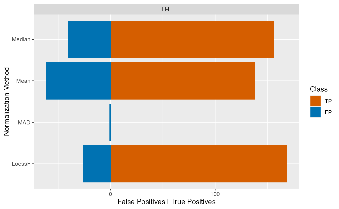

If many pairwise comparisons were performed, the plot_TP_FP_spiked_box() function can be used to visualize the distribution of true and false positives for all pairwise comparisons in a boxplot.

Given that the data set encompasses merely two distinct spike-in concentrations and therefore only one pairwise comparison has been conducted in DE analysis, a barplot would be more appropriate. Nonetheless, for demonstration purposes, a boxplot will be used here.

plot_TP_FP_spiked_box(stats, ain = c("Median", "Mean", "MAD", "LoessF"), comparisons = NULL)
#> All comparisons of stats will be visualized.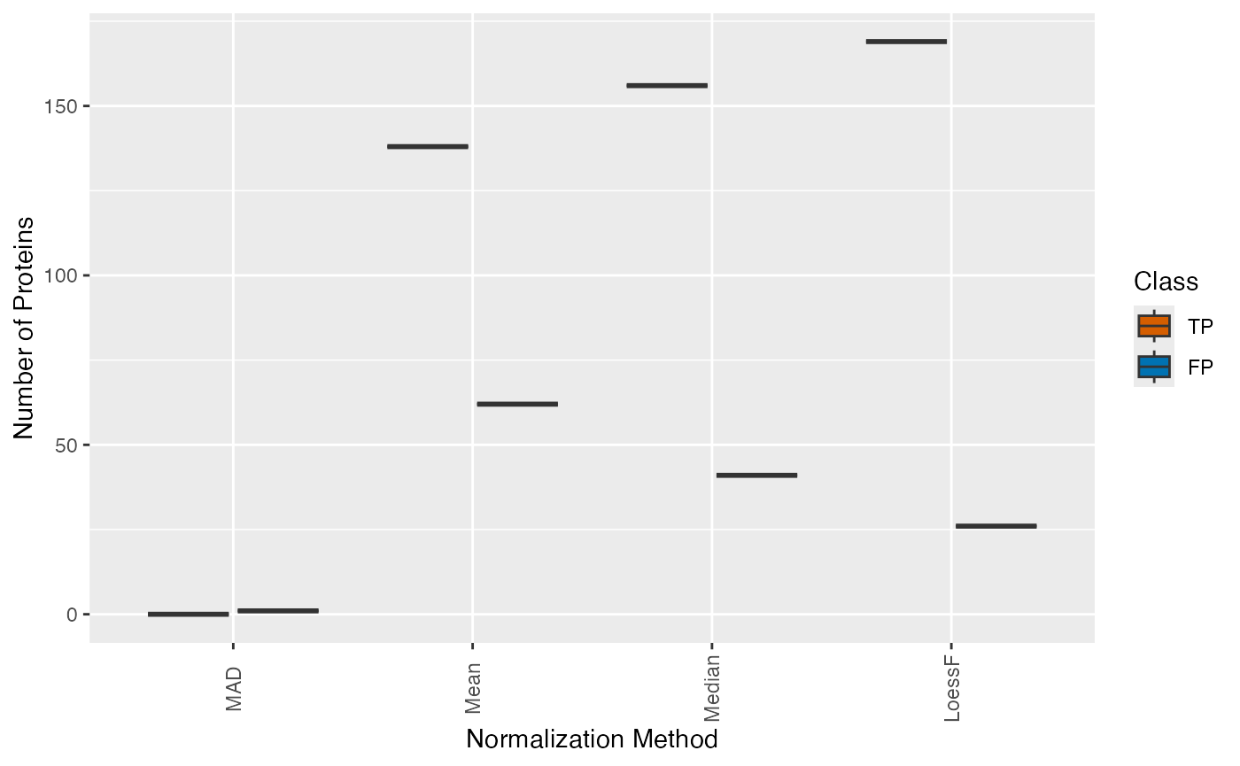

Furthermore, similarly the plot_TP_FP_spiked_scatter() function can be used to visualize the true and false positives in a scatter plot. Here, a scatterplot of the median true positives and false positives is calculated across all comparisons and displayed for each normalization method with errorbars showing the Q1 and Q3. Here again, this plot is more suitable for data sets with multiple pairwise comparisons.

plot_TP_FP_spiked_scatter(stats, ain = NULL, comparisons = NULL)
#> All comparisons of stats will be visualized.
#> All normalization methods of de_res will be visualized.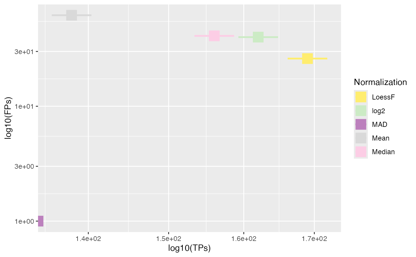

Furthermore, other performance metrics that the number of true positives and false positives can be visualized using the plot_stats_spiked_heatmap() function. Here, currently, the sensitivity, specificity, precision, FPR, F1 score, and accuracy can be visualized for the different normalization methods and pairwise comparisons.

plot_stats_spiked_heatmap(stats, ain = c("Median", "Mean", "MAD"), metrics = c("Precision", "F1Score"))
#> All comparisons of stats will be visualized.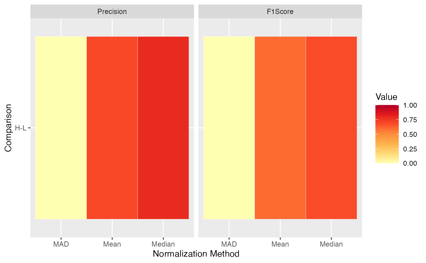

Finally, ROC and AUC values can be calculated and visualized using the plot_ROC_AUC_spiked() function. This function returns a plot showing the ROC curves, a bar plot with the AUC values for each comparison, and a boxplot with the distributions of AUC values across all comparisons.

plot_ROC_AUC_spiked(se_norm, de_res, ain = c("Median", "Mean", "LoessF"), comparisons = NULL)
#> All comparisons of de_res will be visualized.
#> $ROC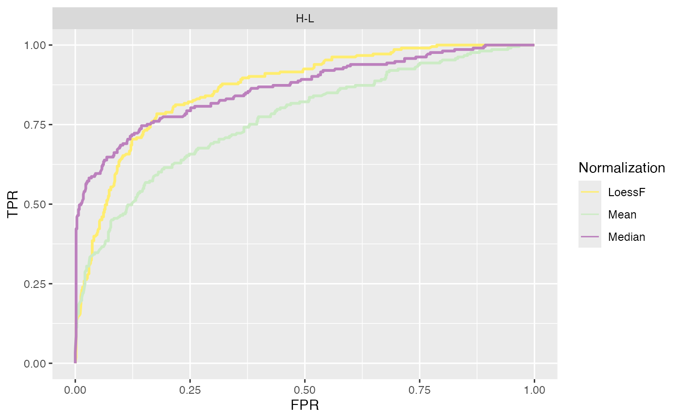

#> 
#> $AUC_bars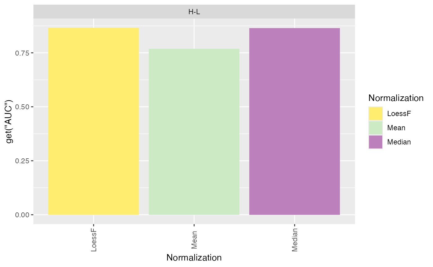

#> 
#> $AUC_box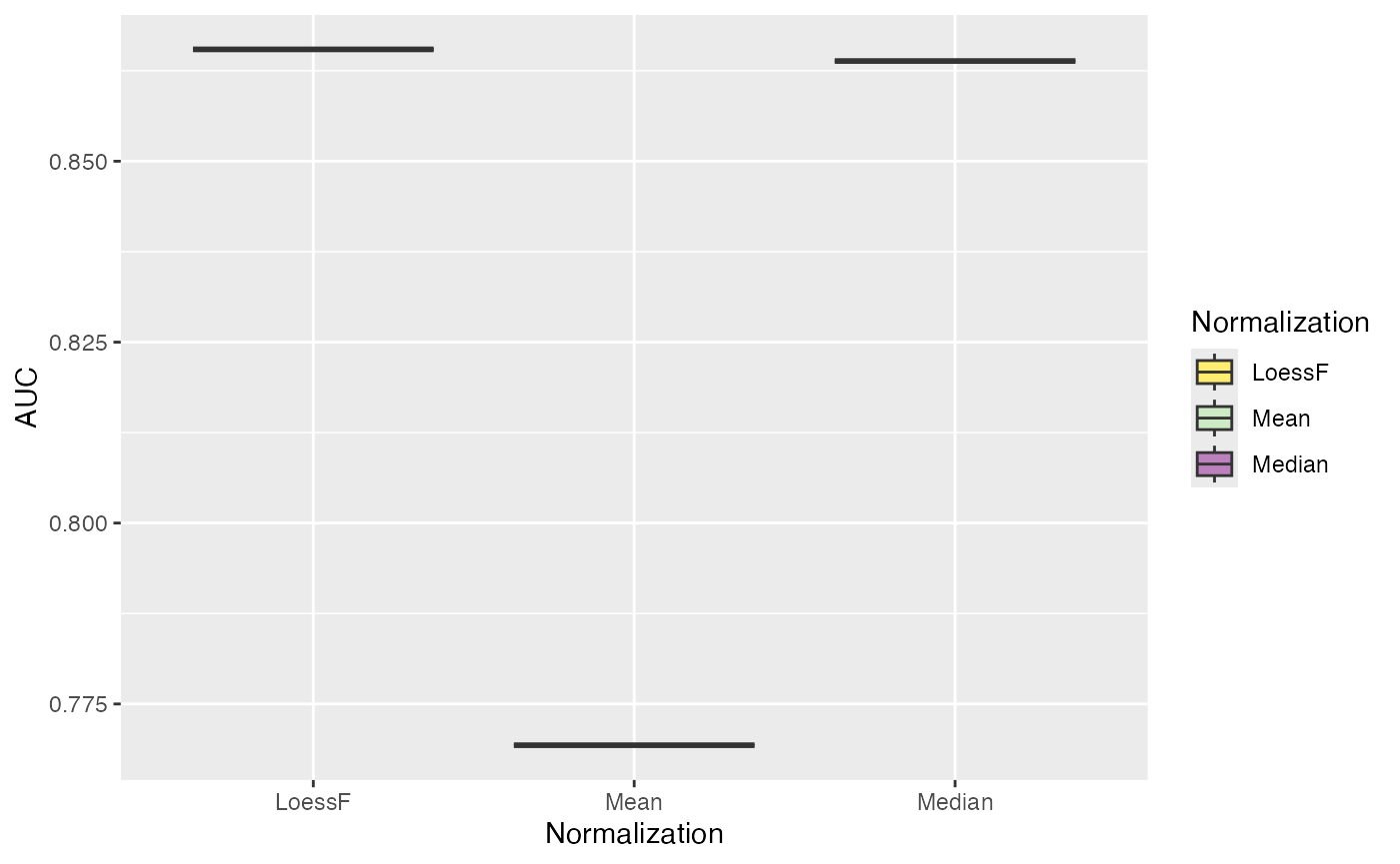

#> 
#> $AUC_dt
#>   PANEL Comparison group  Assay       AUC
#> 1     1        H-L     1 LoessF 0.8654546
#> 2     1        H-L     2   Mean 0.7693012
#> 3     1        H-L     3 Median 0.8638456

Log Fold Change Distributions

Furthermore, you can visualize the distribution of log fold changes for the different conditions using the plot_fold_changes_spiked() function. The fold changes of the background proteins should be centered around zero, while the spike-in proteins should be centered around the actual log fold change calculated based on the spike-in concentrations.

plot_fold_changes_spiked(se_norm, de_res, condition = "Condition", ain = c("Median", "Mean", "MAD"), comparisons = NULL)
#> All comparisons of de_res will be visualized.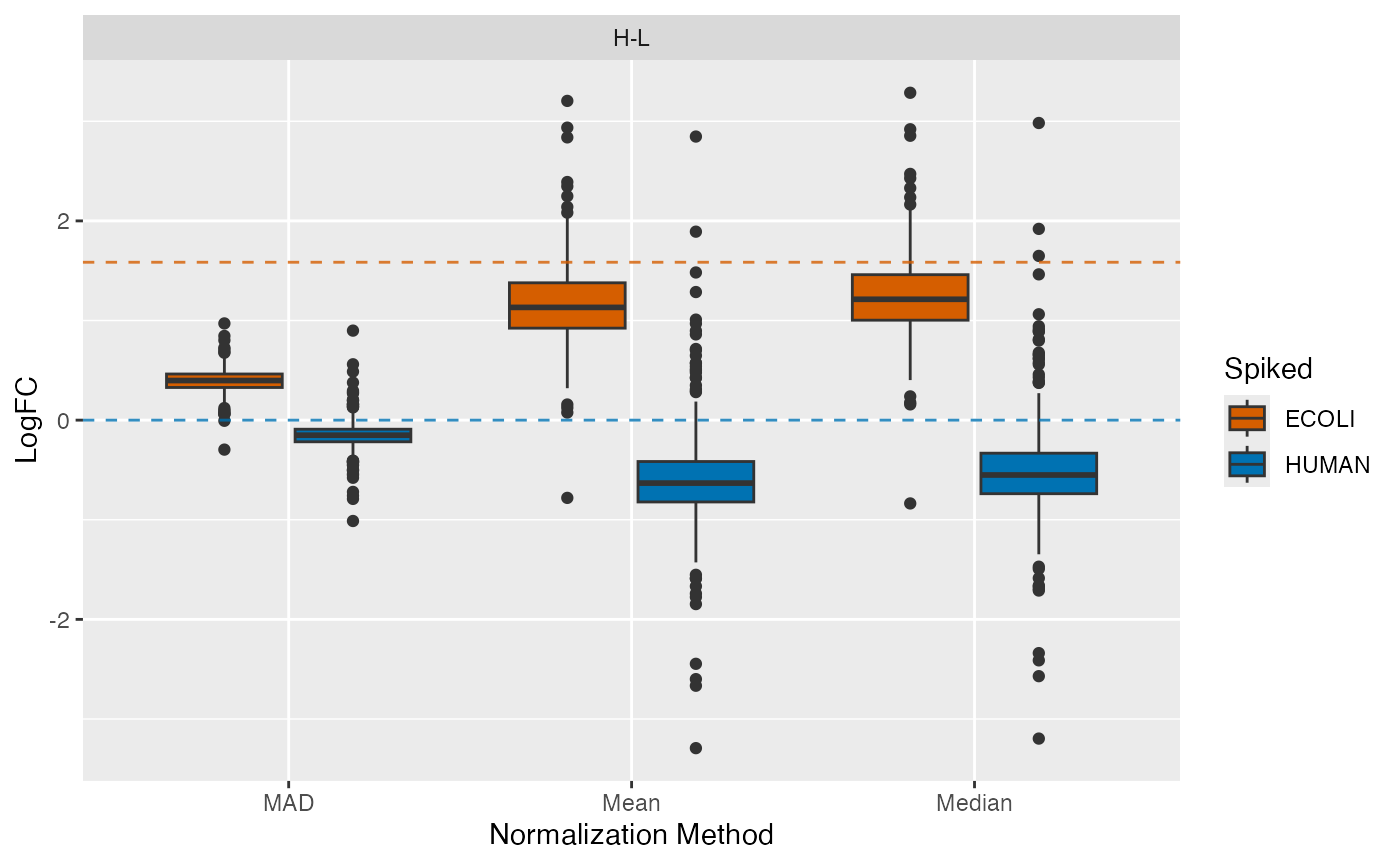

P-Value Distributions

Similarly, the distributions of the p-values can be visualized using the plot_pvalues_spiked() function.

plot_pvalues_spiked(se_norm, de_res, ain = c("Median", "Mean", "MAD"), comparisons = NULL)
#> All comparisons of de_res will be visualized.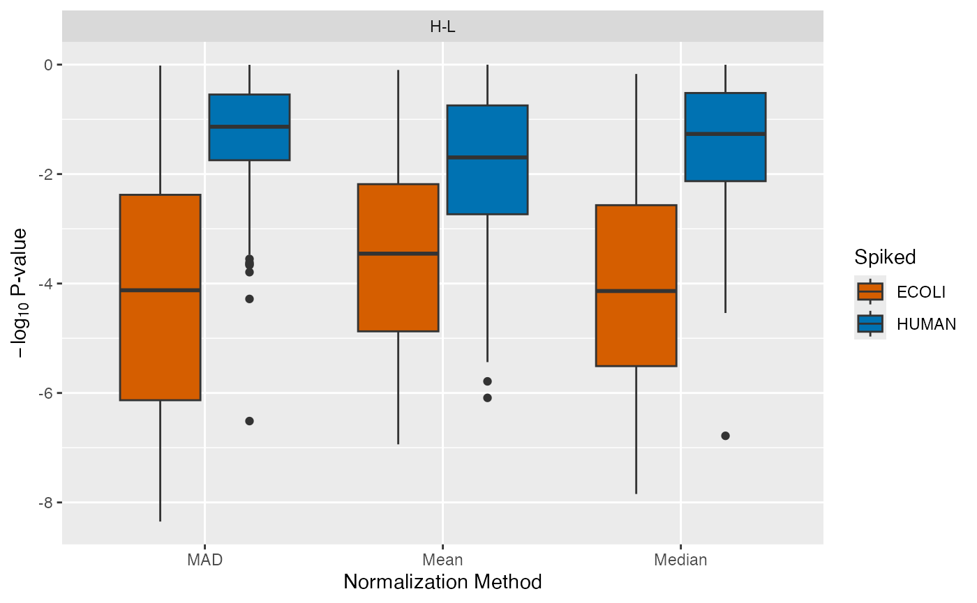

Log Fold Change Thresholds

Due to the high amount of false positives encountered in spike-in data sets, we provided a function to test for different log fold change thresholds to try to reduce the amount of false positives. The function plot_logFC_thresholds_spiked() can be used to visualize the number of true positives and false positives for different log fold change thresholds.

plot_logFC_thresholds_spiked(se_norm, de_res, condition = NULL, ain = c("Median", "Mean", "MAD"), nrow = 1, alpha = 0.05)
#> All comparisons of de_res will be visualized.
#> Condition of SummarizedExperiment used!
#> $TP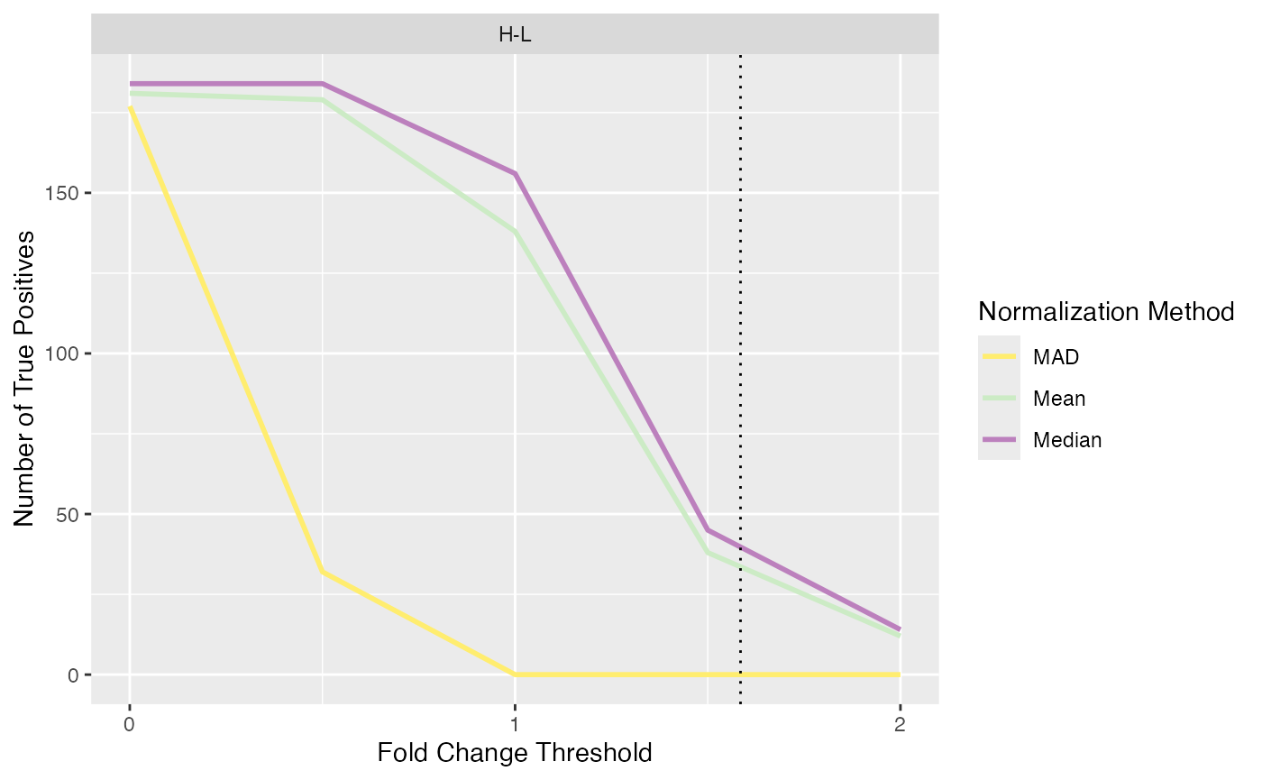

#> 
#> $FP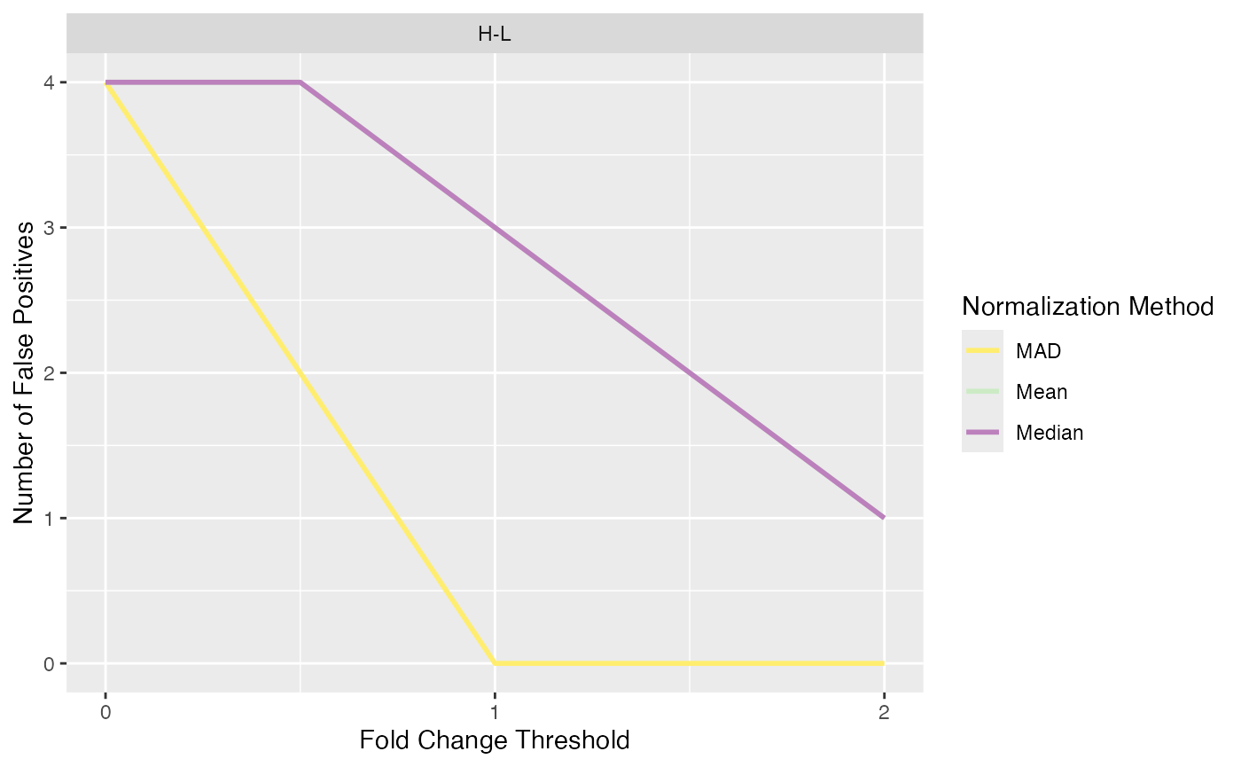

Session Info

utils::sessionInfo()
#> R version 4.4.1 (2024-06-14)
#> Platform: aarch64-apple-darwin20
#> Running under: macOS Sonoma 14.4
#> 
#> Matrix products: default
#> BLAS:   /Library/Frameworks/R.framework/Versions/4.4-arm64/Resources/lib/libRblas.0.dylib 
#> LAPACK: /Library/Frameworks/R.framework/Versions/4.4-arm64/Resources/lib/libRlapack.dylib;  LAPACK version 3.12.0
#> 
#> locale:
#> [1] en_US.UTF-8/en_US.UTF-8/en_US.UTF-8/C/en_US.UTF-8/en_US.UTF-8
#> 
#> time zone: Europe/Berlin
#> tzcode source: internal
#> 
#> attached base packages:
#> [1] stats     graphics  grDevices datasets  utils     methods   base     
#> 
#> other attached packages:
#> [1] PRONE_0.99.6
#> 
#> loaded via a namespace (and not attached):
#>   [1] rlang_1.1.4                 magrittr_2.0.3             
#>   [3] clue_0.3-65                 matrixStats_1.3.0          
#>   [5] compiler_4.4.1              systemfonts_1.1.0          
#>   [7] vctrs_0.6.5                 reshape2_1.4.4             
#>   [9] stringr_1.5.1               ProtGenerics_1.36.0        
#>  [11] pkgconfig_2.0.3             crayon_1.5.3               
#>  [13] fastmap_1.2.0               XVector_0.44.0             
#>  [15] labeling_0.4.3              utf8_1.2.4                 
#>  [17] rmarkdown_2.27              UCSC.utils_1.0.0           
#>  [19] preprocessCore_1.66.0       ragg_1.3.2                 
#>  [21] purrr_1.0.2                 xfun_0.46                  
#>  [23] MultiAssayExperiment_1.30.3 zlibbioc_1.50.0            
#>  [25] cachem_1.1.0                GenomeInfoDb_1.40.1        
#>  [27] jsonlite_1.8.8              highr_0.11                 
#>  [29] DelayedArray_0.30.1         BiocParallel_1.38.0        
#>  [31] parallel_4.4.1              cluster_2.1.6              
#>  [33] R6_2.5.1                    RColorBrewer_1.1-3         
#>  [35] bslib_0.7.0                 stringi_1.8.4              
#>  [37] limma_3.60.4                GenomicRanges_1.56.1       
#>  [39] jquerylib_0.1.4             iterators_1.0.14           
#>  [41] Rcpp_1.0.13                 SummarizedExperiment_1.34.0
#>  [43] knitr_1.48                  IRanges_2.38.1             
#>  [45] splines_4.4.1               Matrix_1.7-0               
#>  [47] igraph_2.0.3                tidyselect_1.2.1           
#>  [49] rstudioapi_0.16.0           abind_1.4-5                
#>  [51] yaml_2.3.10                 ggtext_0.1.2               
#>  [53] doParallel_1.0.17           codetools_0.2-20           
#>  [55] affy_1.82.0                 lattice_0.22-6             
#>  [57] tibble_3.2.1                plyr_1.8.9                 
#>  [59] withr_3.0.0                 Biobase_2.64.0             
#>  [61] evaluate_0.24.0             desc_1.4.3                 
#>  [63] xml2_1.3.6                  pillar_1.9.0               
#>  [65] affyio_1.74.0               BiocManager_1.30.23        
#>  [67] MatrixGenerics_1.16.0       renv_1.0.7                 
#>  [69] foreach_1.5.2               stats4_4.4.1               
#>  [71] MSnbase_2.30.1              MALDIquant_1.22.2          
#>  [73] ncdf4_1.22                  generics_0.1.3             
#>  [75] S4Vectors_0.42.1            ggplot2_3.5.1              
#>  [77] munsell_0.5.1               scales_1.3.0               
#>  [79] glue_1.7.0                  lazyeval_0.2.2             
#>  [81] tools_4.4.1                 data.table_1.15.4          
#>  [83] mzID_1.42.0                 QFeatures_1.14.2           
#>  [85] vsn_3.72.0                  mzR_2.38.0                 
#>  [87] fs_1.6.4                    XML_3.99-0.17              
#>  [89] grid_4.4.1                  impute_1.78.0              
#>  [91] tidyr_1.3.1                 MsCoreUtils_1.16.0         
#>  [93] colorspace_2.1-0            GenomeInfoDbData_1.2.12    
#>  [95] PSMatch_1.8.0               cli_3.6.3                  
#>  [97] textshaping_0.4.0           plotROC_2.3.1              
#>  [99] fansi_1.0.6                 S4Arrays_1.4.1             
#> [101] dplyr_1.1.4                 AnnotationFilter_1.28.0    
#> [103] pcaMethods_1.96.0           gtable_0.3.5               
#> [105] sass_0.4.9                  digest_0.6.36              
#> [107] BiocGenerics_0.50.0         SparseArray_1.4.8          
#> [109] farver_2.1.2                htmlwidgets_1.6.4          
#> [111] htmltools_0.5.8.1           pkgdown_2.1.0              
#> [113] lifecycle_1.0.4             httr_1.4.7                 
#> [115] NormalyzerDE_1.22.0         statmod_1.5.0              
#> [117] gridtext_0.1.5              MASS_7.3-61

References

Cox, Jürgen, Marco Y. Hein, Christian A. Luber, Igor Paron, Nagarjuna Nagaraj, and Matthias Mann. 2014. “Accurate Proteome-Wide Label-Free Quantification by Delayed Normalization and Maximal Peptide Ratio Extraction, Termed Maxlfq.” Molecular & Cellular Proteomics 13 (9): 2513–26. https://doi.org/10.1074/mcp.M113.031591.

Arend Lis