Differential Expression Analysis

library(PRONE)

Load Data (TMT)

Here, we are directly working with the SummarizedExperiment data. For more information on how to create the SummarizedExperiment from a proteomics data set, please refer to the “Get Started” vignette.

The example TMT data set originates from (Biadglegne et al. 2022).

data("tuberculosis_TMT_se")
se <- tuberculosis_TMT_se

Normalize Data

In order to compare the performance of different normalization methods on their ability to detect differentially expressed proteins, we first perform a simple normalization here. For more details about how to normalize data and evaluate the normalization appraoches quantitatively and qualitatively using PRONE, please refer to the “Normalization” vignette.

se_norm <- normalize_se(se, c("IRS_on_RobNorm", "IRS_on_Median", "IRS_on_LoessF", "IRS_on_Quantile"), combination_pattern = "_on_")
#> RobNorm normalization not yet performed. Single RobNorm normalization performed now.
#> RobNorm completed.
#> IRS normalization performed on RobNorm-normalized data completed.
#> Median normalization not yet performed. Single Median normalization performed now.
#> Median completed.
#> IRS normalization performed on Median-normalized data completed.
#> LoessF normalization not yet performed. Single LoessF normalization performed now.
#> LoessF completed.
#> IRS normalization performed on LoessF-normalized data completed.
#> Quantile normalization not yet performed. Single Quantile normalization performed now.
#> Quantile completed.
#> IRS normalization performed on Quantile-normalized data completed.

After having performed normalization and evaluated the different normalization methods via qualitative and quantitative analysis, differential expression analysis can be used to further analyze the differences of the normalization methods.

However before, you need to remove the reference samples in case of a TMT experiment. This can be easily done with the function remove_reference_samples().

se_norm <- remove_reference_samples(se_norm)
#> 2 reference samples removed from the SummarizedExperiment object.

Run DE Analysis

First, you need to specify the comparisons you want to perform in DE analysis. For this, the function specifc_comparisons() was developed which helps to build the right comparison strings. For instance, if you are having a condition column “Condition” in your meta data that is built upon two individual groups, such as “diabetic_3d” referring to diabetic samples at day 3 after operation, you can simply specify sep = “_” and the method only considers comparisons where at least one of the group remains static.

However, you can also just simply create a vector of comparisons to ensure the correct order and handle this vector over to the DE analysis method.

comparisons <- specify_comparisons(se_norm, condition = "Group", sep = NULL, control = NULL)

comparisons <- c("PTB-HC", "TBL-HC", "TBL-PTB", "Rx-PTB")

The function run_DE() performs the DE analysis on the selected SummarizedExperiment and comparisons. DE analysis can be performed on multiple assays (normalization methods) at once using the already known “ain” parameter. The condition of the SummarizedExperiment object, specified at the beginning, can be used (condition = NULL) or any other column of the meta data can specified. Three methods are available for DE analysis: limma (Ritchie et al. 2015), DEqMS (Zhu et al. 2020), and ROTS (Suomi et al. 2017). The meaning of the other parameters can be extracted from the documentation of the method.

de_res <- run_DE(se = se_norm, 
                     comparisons = comparisons,
                     ain = NULL, 
                     condition = NULL, 
                     DE_method = "limma", 
                     covariate = NULL, 
                     logFC = TRUE, 
                     logFC_up = 1, 
                     logFC_down = -1, 
                     p_adj = TRUE, 
                     alpha = 0.05,
                     trend = TRUE,
                     robust = TRUE,
                 ) 
#> Condition of SummarizedExperiment used!
#> All assays of the SummarizedExperiment will be used.
#> DE Analysis will not be performed on raw data.
#> log2: DE analysis completed.
#> RobNorm: DE analysis completed.
#> IRS_on_RobNorm: DE analysis completed.
#> Median: DE analysis completed.
#> IRS_on_Median: DE analysis completed.
#> LoessF: DE analysis completed.
#> IRS_on_LoessF: DE analysis completed.
#> Quantile: DE analysis completed.
#> IRS_on_Quantile: DE analysis completed.

When running ROTS you need to specify the R and K parameters. In DEqMS, the DEqMS_PSMs_column need to be specified. This can be any column in the rowData(se). For more information on the specific parameters, please refer to the method specific documentation.

If you want to apply other logFC or p-value threshold, there is no need to re-run the DE analysis again. With apply_thresholds(), you can simply change the threshold values.

new_de_res <- apply_thresholds(de_res = de_res, logFC = FALSE, p_adj = TRUE, alpha = 0.05)

Visualize DE Results

Barplot

To get an overview of the DE results of the different normalization methods, you can visualize the number of significant DE proteins per normalization method in a barplot using plot_overview_DE_bar(). This plot can be generated in different ways by specifying the “plot_type” parameter:

single: plot a single barplot for each comparison (default)
facet_comp: facet the barplot by comparison
stacked: stack the number of DE per comparison
facet_regulation: stack the number of DE per comparison but facet by up- and down-regulated

plot_overview_DE_bar(de_res, ain = NULL, comparisons = comparisons, plot_type = "facet_regulation") + ggplot2::theme(legend.position = "bottom", legend.direction = "vertical")
#> All normalization methods of de_res will be visualized.

You can also just visualize two specific comparisons:

plot_overview_DE_bar(de_res, ain = NULL, comparisons = comparisons[seq_len(2)], plot_type = "facet_comp")
#> All normalization methods of de_res will be visualized.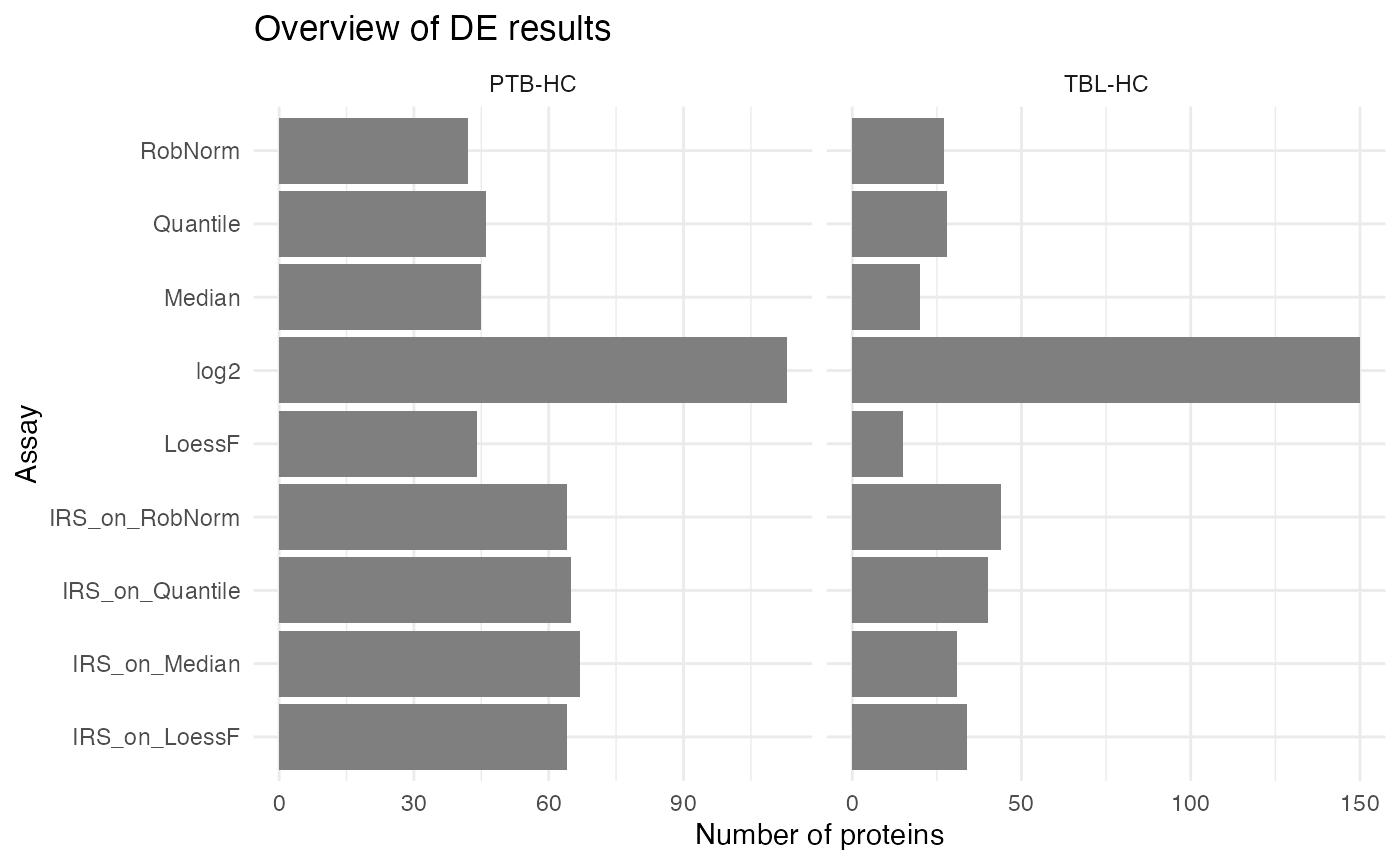

Tile Plot

You can also get an overview of the DE results in form of a heatmap using the plot_overview_DE_tile().

plot_overview_DE_tile(de_res)
#> All comparisons of de_res will be visualized.
#> All normalization methods of de_res will be visualized.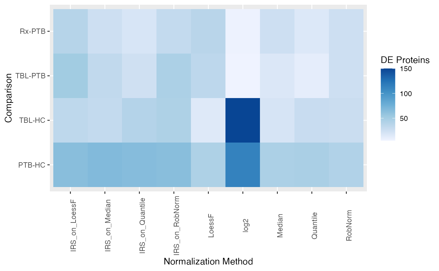

Volcano Plots

Another option is to generate volcano plots for each comparison. The function plot_volcano_DE() generates a grid of volcano plots for each normalization techniques (facet_norm = TRUE) or for each comparison (facet_comparison = TRUE). A list of volcano plots is returned.

plot_volcano_DE(de_res, ain = NULL, comparisons = comparisons[1], facet_norm = TRUE)
#> All normalization methods of de_res will be visualized.
#> $`PTB-HC`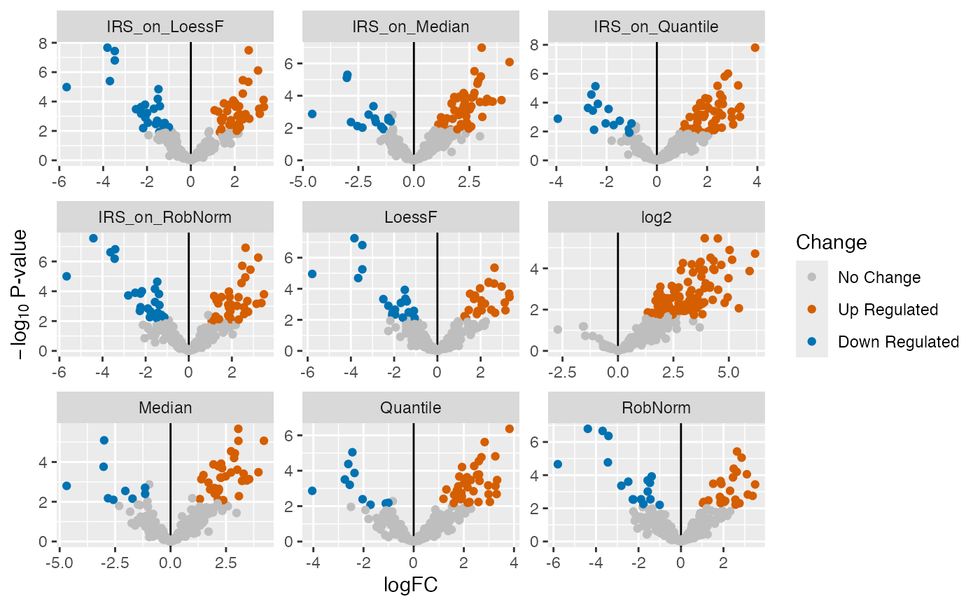

Heatmap of DE Results

Furthermore, you can visualize the DE results in form of a heatmap. The function plot_heatmap_DE() generates a heatmap of the DE results for a specific comparison and normalization method.

plot_heatmap_DE(tuberculosis_TMT_se, tuberculosis_TMT_de_res, ain = NULL, comparison = "PTB-HC", condition = NULL, label_by = NULL, pvalue_column = "adj.P.Val")
#> All assays of the SummarizedExperiment will be used.
#> Label of SummarizedExperiment used!
#> Condition of SummarizedExperiment used!
#> <simpleError in stats::hclust(stats::dist(as.matrix(data))): NA/NaN/Inf in foreign function call (arg 10)>
#> <simpleError in stats::hclust(stats::dist(as.matrix(data))): NA/NaN/Inf in foreign function call (arg 10)>
#> <simpleError in stats::hclust(stats::dist(as.matrix(data))): NA/NaN/Inf in foreign function call (arg 10)>
#> <simpleError in stats::hclust(stats::dist(as.matrix(data))): NA/NaN/Inf in foreign function call (arg 10)>
#> <simpleError in stats::hclust(stats::dist(as.matrix(data))): NA/NaN/Inf in foreign function call (arg 10)>
#> $log2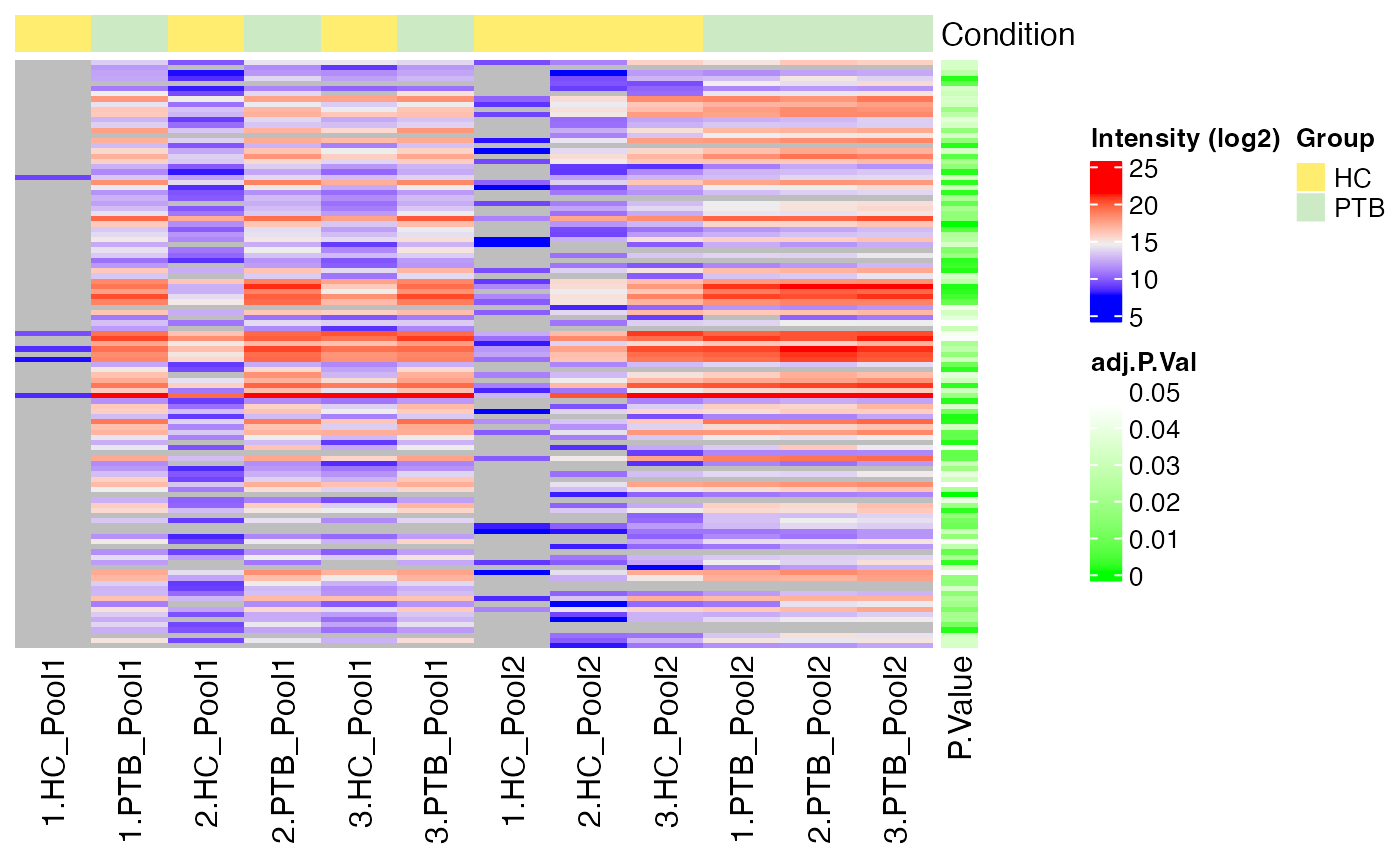

#> 
#> $RobNorm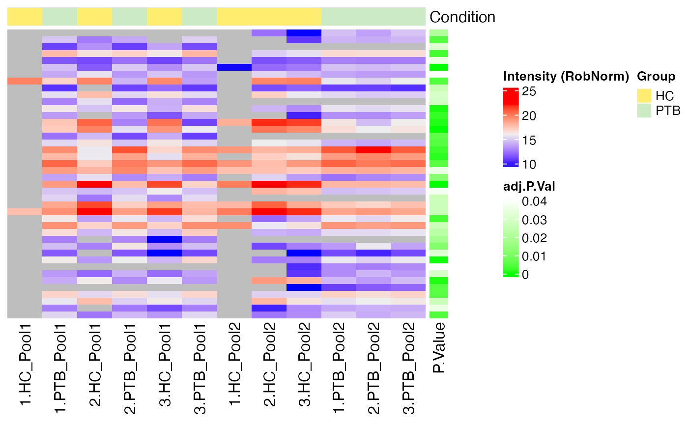

#> 
#> $IRS_on_RobNorm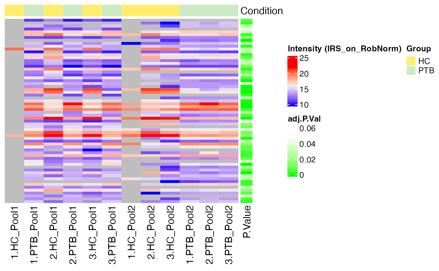

#> 
#> $Median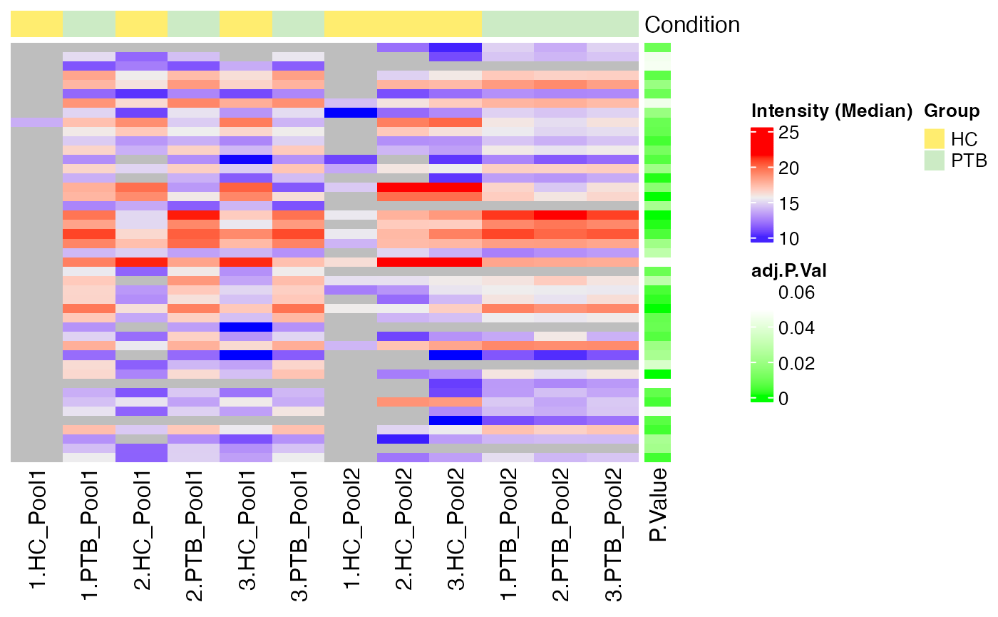

#> 
#> $IRS_on_Median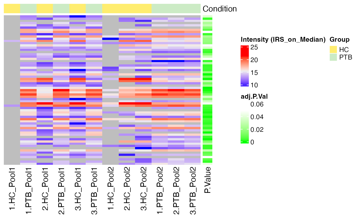

Coverage of Biomarkers

In case you know some biomarkers of previous publications that should be significantly expressed in your biological context, you can check the number of specified markers that are DE in the different normalization methods.

TODO: plot_coverage_DE_bar

Intersection Analysis of DE Results

Moreover, you can also intersect the DE results of different normalization methods to see how many DE proteins overlap. You can either plot for each requested comparison an individual upset plot (plot_type = “single”) or stack the number of overlapping DE proteins per comparison (“stacked”). Not only the upset plot(s) are returned, but also a table with the intersections is provided by the plot_upset_DE()function.

intersections <- plot_upset_DE(de_res, ain = NULL, comparisons = comparisons[seq_len(3)], min_degree = 6, plot_type = "stacked")
#> All normalization methods of de_res will be visualized.
# put legend on top due to very long comparisons
intersections$upset[[2]] <- intersections$upset[[2]] + ggplot2::theme(legend.position = "top", legend.direction = "vertical")
intersections$upset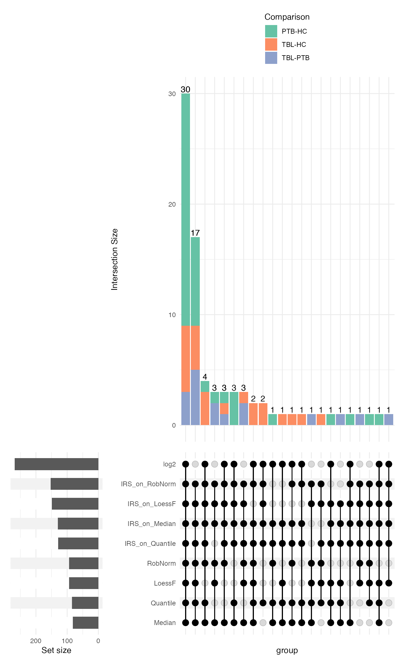

Additionally, the Jaccard similarity index can be calculated to quantify the similarity of the DE results between the different normalization methods. A individual heatmap can be generated for each comparison (“plot_type = single”), a single heatmap facetted by comparison (“facet_comp”) or a single heatmap taking all comparisons into account (“all”) can be generated.

plot_jaccard_heatmap(de_res, ain = NULL, comparisons = comparisons, plot_type = "all")
#> All normalization methods of de_res will be visualized.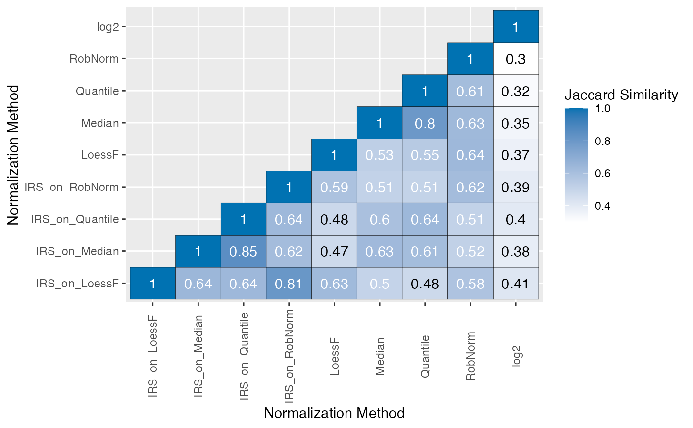

PRONE offers the functionality to extract a consensus set of DEPs based on a selection of normalization methods and a threshold for the number of methods that need to agree on the DE status of a protein. The function get_consensus_DE() returns a list of consensus DE proteins for either each comparison separately or for all comparisons combined.

DT::datatable(extract_consensus_DE_candidates(de_res, ain = NULL, comparisons = comparisons, norm_thr = 0.8, per_comparison = TRUE), options = list(scrollX = TRUE))

Session Info

utils::sessionInfo()
#> R version 4.4.1 (2024-06-14)
#> Platform: aarch64-apple-darwin20
#> Running under: macOS Sonoma 14.4
#> 
#> Matrix products: default
#> BLAS:   /Library/Frameworks/R.framework/Versions/4.4-arm64/Resources/lib/libRblas.0.dylib 
#> LAPACK: /Library/Frameworks/R.framework/Versions/4.4-arm64/Resources/lib/libRlapack.dylib;  LAPACK version 3.12.0
#> 
#> locale:
#> [1] en_US.UTF-8/en_US.UTF-8/en_US.UTF-8/C/en_US.UTF-8/en_US.UTF-8
#> 
#> time zone: Europe/Berlin
#> tzcode source: internal
#> 
#> attached base packages:
#> [1] stats     graphics  grDevices datasets  utils     methods   base     
#> 
#> other attached packages:
#> [1] PRONE_0.99.6
#> 
#> loaded via a namespace (and not attached):
#>   [1] rlang_1.1.4                 magrittr_2.0.3             
#>   [3] GetoptLong_1.0.5            clue_0.3-65                
#>   [5] matrixStats_1.3.0           compiler_4.4.1             
#>   [7] png_0.1-8                   systemfonts_1.1.0          
#>   [9] vctrs_0.6.5                 reshape2_1.4.4             
#>  [11] stringr_1.5.1               ProtGenerics_1.36.0        
#>  [13] shape_1.4.6.1               pkgconfig_2.0.3            
#>  [15] crayon_1.5.3                fastmap_1.2.0              
#>  [17] XVector_0.44.0              labeling_0.4.3             
#>  [19] utf8_1.2.4                  rmarkdown_2.27             
#>  [21] UCSC.utils_1.0.0            preprocessCore_1.66.0      
#>  [23] ragg_1.3.2                  purrr_1.0.2                
#>  [25] xfun_0.46                   MultiAssayExperiment_1.30.3
#>  [27] zlibbioc_1.50.0             cachem_1.1.0               
#>  [29] GenomeInfoDb_1.40.1         jsonlite_1.8.8             
#>  [31] highr_0.11                  DelayedArray_0.30.1        
#>  [33] BiocParallel_1.38.0         parallel_4.4.1             
#>  [35] cluster_2.1.6               R6_2.5.1                   
#>  [37] RColorBrewer_1.1-3          bslib_0.7.0                
#>  [39] stringi_1.8.4               ComplexUpset_1.3.3         
#>  [41] limma_3.60.4                GenomicRanges_1.56.1       
#>  [43] jquerylib_0.1.4             iterators_1.0.14           
#>  [45] Rcpp_1.0.13                 SummarizedExperiment_1.34.0
#>  [47] knitr_1.48                  IRanges_2.38.1             
#>  [49] splines_4.4.1               Matrix_1.7-0               
#>  [51] igraph_2.0.3                tidyselect_1.2.1           
#>  [53] rstudioapi_0.16.0           abind_1.4-5                
#>  [55] yaml_2.3.10                 ggtext_0.1.2               
#>  [57] doParallel_1.0.17           codetools_0.2-20           
#>  [59] affy_1.82.0                 lattice_0.22-6             
#>  [61] tibble_3.2.1                plyr_1.8.9                 
#>  [63] withr_3.0.0                 Biobase_2.64.0             
#>  [65] evaluate_0.24.0             desc_1.4.3                 
#>  [67] xml2_1.3.6                  circlize_0.4.16            
#>  [69] pillar_1.9.0                affyio_1.74.0              
#>  [71] BiocManager_1.30.23         MatrixGenerics_1.16.0      
#>  [73] DT_0.33                     renv_1.0.7                 
#>  [75] foreach_1.5.2               stats4_4.4.1               
#>  [77] MSnbase_2.30.1              MALDIquant_1.22.2          
#>  [79] ncdf4_1.22                  generics_0.1.3             
#>  [81] S4Vectors_0.42.1            ggplot2_3.5.1              
#>  [83] munsell_0.5.1               scales_1.3.0               
#>  [85] glue_1.7.0                  lazyeval_0.2.2             
#>  [87] tools_4.4.1                 data.table_1.15.4          
#>  [89] mzID_1.42.0                 QFeatures_1.14.2           
#>  [91] vsn_3.72.0                  mzR_2.38.0                 
#>  [93] fs_1.6.4                    XML_3.99-0.17              
#>  [95] grid_4.4.1                  impute_1.78.0              
#>  [97] tidyr_1.3.1                 crosstalk_1.2.1            
#>  [99] MsCoreUtils_1.16.0          colorspace_2.1-0           
#> [101] patchwork_1.2.0             GenomeInfoDbData_1.2.12    
#> [103] PSMatch_1.8.0               cli_3.6.3                  
#> [105] textshaping_0.4.0           fansi_1.0.6                
#> [107] S4Arrays_1.4.1              ComplexHeatmap_2.20.0      
#> [109] dplyr_1.1.4                 AnnotationFilter_1.28.0    
#> [111] pcaMethods_1.96.0           gtable_0.3.5               
#> [113] sass_0.4.9                  digest_0.6.36              
#> [115] BiocGenerics_0.50.0         SparseArray_1.4.8          
#> [117] rjson_0.2.21                farver_2.1.2               
#> [119] htmlwidgets_1.6.4           htmltools_0.5.8.1          
#> [121] pkgdown_2.1.0               lifecycle_1.0.4            
#> [123] httr_1.4.7                  GlobalOptions_0.1.2        
#> [125] statmod_1.5.0               gridtext_0.1.5             
#> [127] MASS_7.3-61

References

Biadglegne, Fantahun, Johannes R. Schmidt, Kathrin M. Engel, Jörg Lehmann, Robert T. Lehmann, Anja Reinert, Brigitte König, Jürgen Schiller, Stefan Kalkhof, and Ulrich Sack. 2022. “Mycobacterium Tuberculosis Affects Protein and Lipid Content of Circulating Exosomes in Infected Patients Depending on Tuberculosis Disease State.” Biomedicines 10 (4): 783. https://doi.org/10.3390/biomedicines10040783.

Ritchie, Matthew E., Belinda Phipson, Di Wu, Yifang Hu, Charity W. Law, Wei Shi, and Gordon K. Smyth. 2015. “Limma Powers Differential Expression Analyses for Rna-Sequencing and Microarray Studies.” Nucleic Acids Research 43 (7): e47–47. https://doi.org/10.1093/nar/gkv007.

Suomi, Tomi, Fatemeh Seyednasrollah, Maria K. Jaakkola, Thomas Faux, and Laura L. Elo. 2017. “ROTS: An R Package for Reproducibility-Optimized Statistical Testing.” Edited by Timothée Poisot. PLOS Computational Biology 13 (5): e1005562. https://doi.org/10.1371/journal.pcbi.1005562.

Zhu, Yafeng, Lukas M. Orre, Yan Zhou Tran, Georgios Mermelekas, Henrik J. Johansson, Alina Malyutina, Simon Anders, and Janne Lehtiö. 2020. “Deqms: A Method for Accurate Variance Estimation in Differential Protein Expression Analysis.” Molecular & Cellular Proteomics 19 (6): 1047–57. https://doi.org/10.1074/mcp.TIR119.001646.

Differential Expression Analysis

Arend Lis

Load Data (TMT)

Normalize Data