Load Data (TMT)
Here, we are directly working with the SummarizedExperiment data. For more information on how to create the SummarizedExperiment from a proteomics data set, please refer to the “Get Started” vignette.
The example TMT data set originates from (Biadglegne et al. 2022).
data("tuberculosis_TMT_se")
se <- tuberculosis_TMT_se
Normalization
For normalization, there are multiple functions available which can be used to normalize the data. First of all, to know which normalization methods can be applied:
get_normalization_methods()
#>  [1] "GlobalMean"    "GlobalMedian"  "Median"        "Mean"
#>  [5] "IRS"           "Quantile"      "VSN"           "LoessF"
#>  [9] "LoessCyc"      "RLR"           "RlrMA"         "RlrMACyc"
#> [13] "EigenMS"       "MAD"           "RobNorm"       "TMM"
#> [17] "limBE"         "NormicsVSN"    "NormicsMedian"
You can use normalize_se() by specifying all
normalization methods you want to apply on the data. For instance, if
you want to perform median, mean, and MAD normalization, just execute
this line:
se_norm <- normalize_se(se, c("RobNorm", "Mean", "Median"), combination_pattern = NULL)
#> RobNorm completed.
#> Mean completed.
#> Median completed.
However, you can directly also add combinations of methods. The combination pattern specifies which method to apply on top of the specified normalized data. For instance, if you want to perform IRS on top of Median-normalized data:
se_norm <- normalize_se(se, c("RobNorm", "Mean", "Median", "IRS_on_RobNorm", "IRS_on_Mean", "IRS_on_Median"), combination_pattern = "_on_")
#> RobNorm completed.
#> Mean completed.
#> Median completed.
#> IRS normalization performed on RobNorm-normalized data completed.
#> IRS normalization performed on Mean-normalized data completed.
#> IRS normalization performed on Median-normalized data completed.
Finally, you can also normalize your data by applying the specific
normalization method. This makes it possible to design the parameters of
an individual function more specifically. For instance, if you want to
normalize the data by the median, you can use the function
medianNorm(). By default, median normalization is performed
on raw-data. Using the individual normalization functions, you can
easily specify
se_norm <- medianNorm(se_norm, ain = "log2", aout = "Median")All normalized intensities are stored in the SummarizedExperiment object and you can check the already performed normalization techniques using:
names(SummarizedExperiment::assays(se_norm))
#> [1] "raw"            "log2"           "RobNorm"        "Mean"
#> [5] "Median"         "IRS_on_RobNorm" "IRS_on_Mean"    "IRS_on_Median"
We suggest using the default value of the on_raw parameter. This parameter specifies whether the data should be normalized on raw or log2-transformed data. The default value of the “on_raw” parameters was made for each normalization method individually based on publications.
Qualitative and Quantitative Evaluation
PRONE offers many functions to comparatively evaluate the performance of the normalization methods. Notably, the parameter “ain” can always be set. By specifying “ain = NULL”, all normalization methods that were previously performed and are saved in the SummarizedExperiment object are considered. If you want to evaluate only a selection of normalization methods, you can specify them in the “ain” parameter. For instance, if you want to evaluate only the IRS_on_RobNorm and Mean normalization methods, you can set “ain = c(”IRS_on_RobNorm”, “Mean”)“.
Visual Inspection
You can comparatively visualize the normalized data by using the
function plot_boxplots(), plot_densities(),
and plot_pca().
Boxplots of Normalized Data
plot_boxplots(se_norm, ain = NULL, color_by = NULL, label_by = NULL, ncol = 3, facet_norm = TRUE) + ggplot2::theme(legend.position = "bottom", legend.direction = "vertical")
#> All assays of the SummarizedExperiment will be used.
#> Condition of SummarizedExperiment used!
#> Label of SummarizedExperiment used!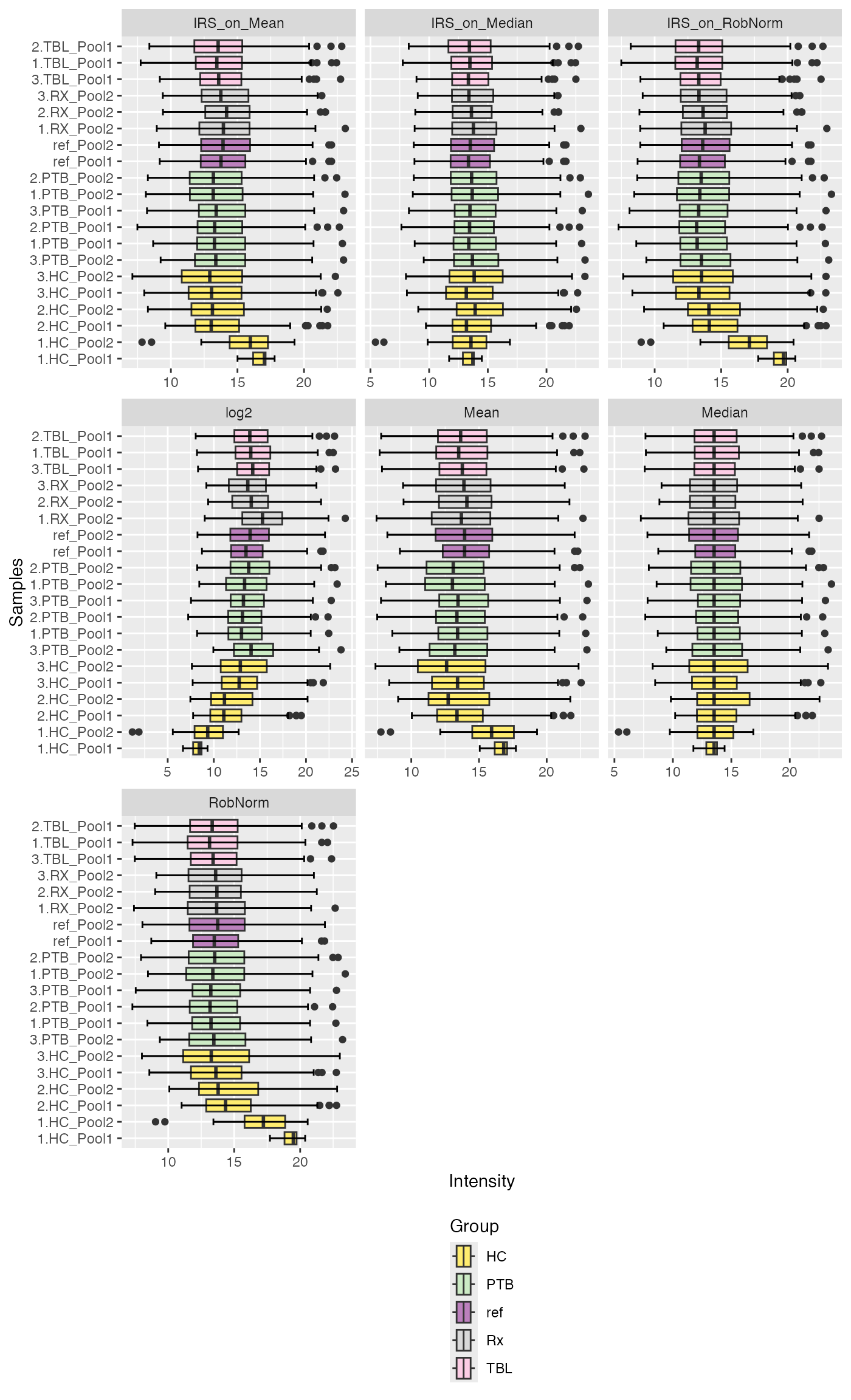
But you can also just plot a selection of normalization methods and color for instance by batch:
plot_boxplots(se_norm, ain = c("IRS_on_RobNorm", "IRS_on_Median"), color_by = "Pool", label_by = NULL, facet_norm = TRUE)
#> Label of SummarizedExperiment used!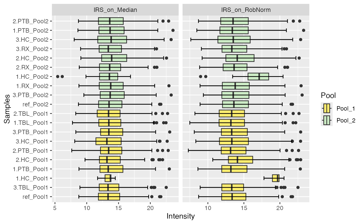
Another option that you have is to return the boxplots for each normalized data independently as a single ggplot object. For this, you need to set facet = FALSE:
plot_boxplots(se_norm, ain = c("IRS_on_RobNorm", "IRS_on_Median"), color_by = "Pool", label_by = NULL, facet_norm = FALSE)
#> Label of SummarizedExperiment used!
#> $IRS_on_RobNorm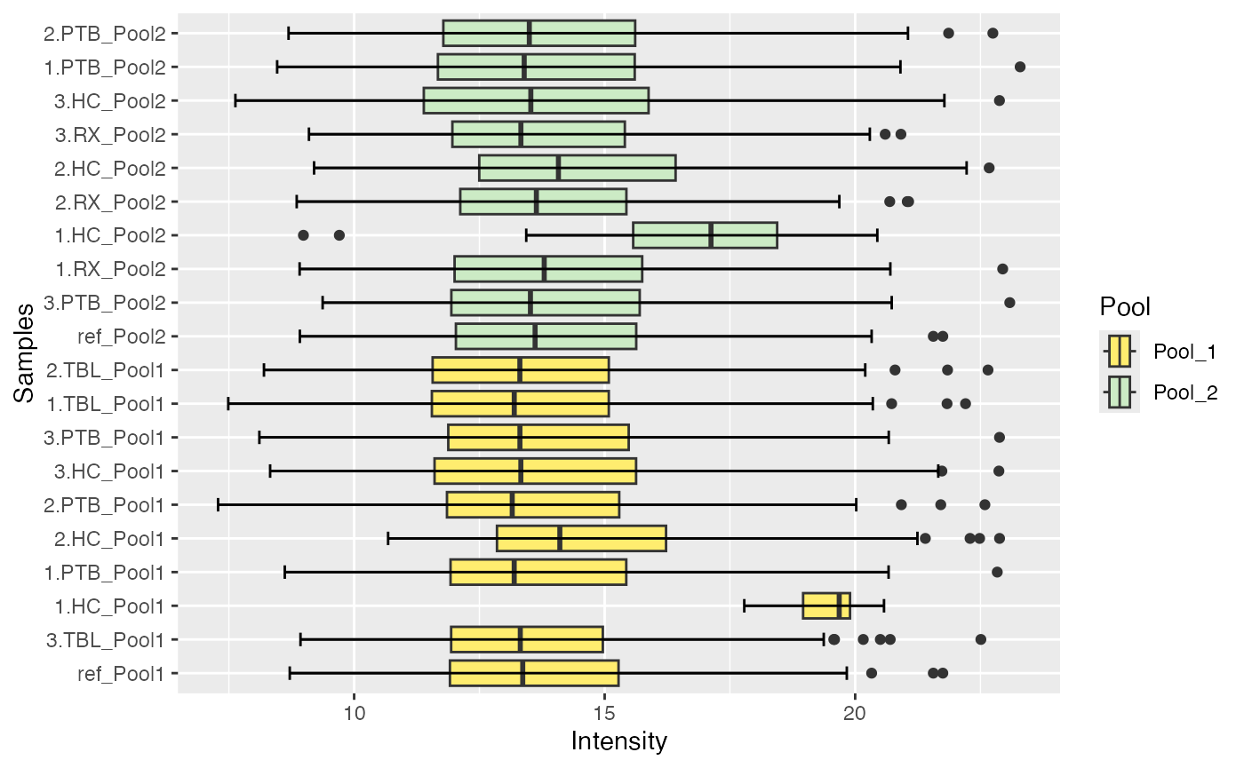
#>
#> $IRS_on_Median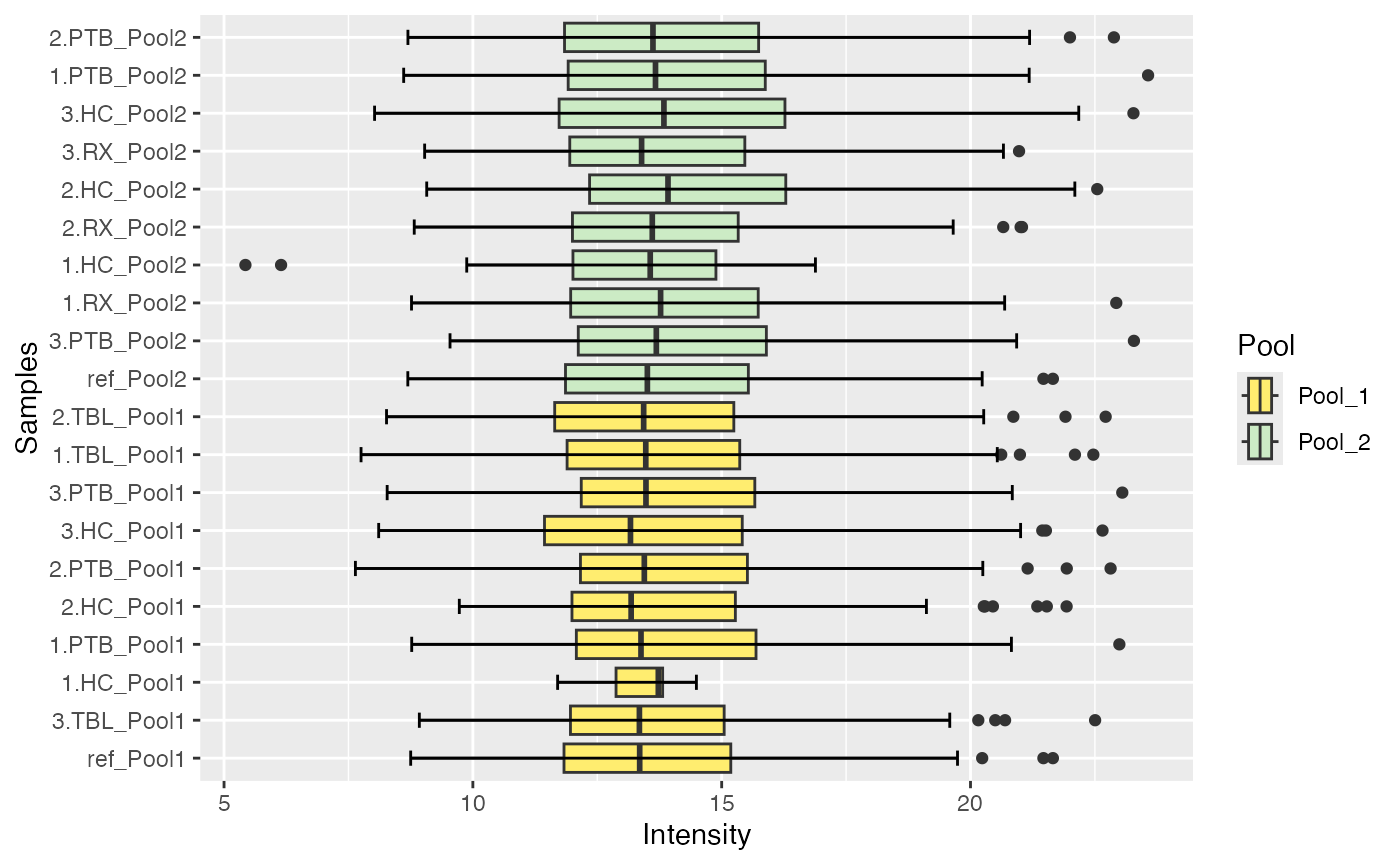
Densities of Normalized Data
Similarly you can visualize the densities of the normalized data.
plot_densities(se_norm, ain = c("IRS_on_RobNorm", "IRS_on_Median"), color_by = NULL, facet_norm = TRUE)
#> Condition of SummarizedExperiment used!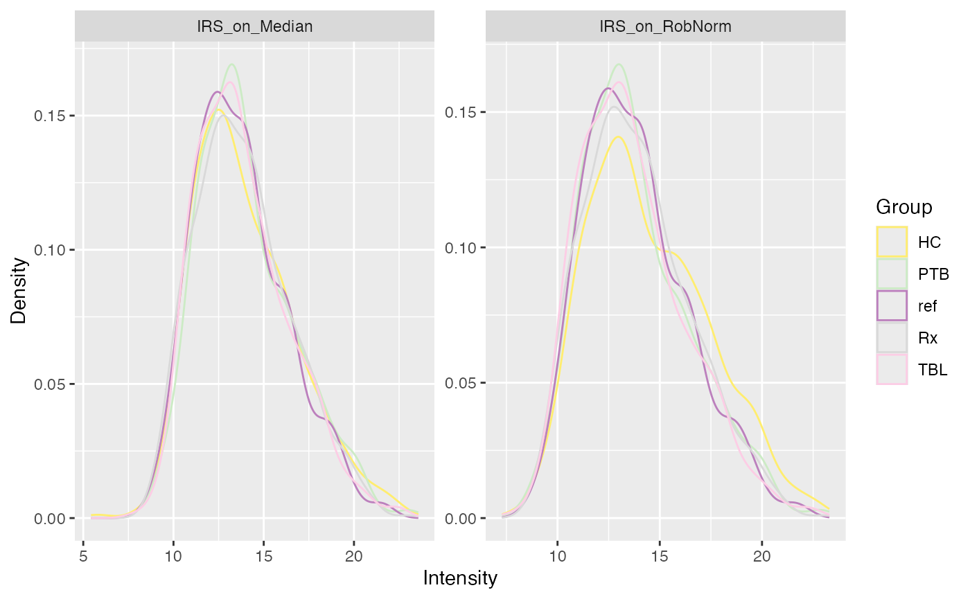
PCA of Normalized Data
Furthermore, you can visualize the normalized data in a PCA plot. Here you have some more arguments that can be specified If you decide to visualize the methods in independent plots (facet_norm = FALSE), then a list of ggplot objects is returned. However, you have the additional option to facet by any other column of the metadata (using the facet_by parameter). Here an example:
plot_PCA(se_norm, ain = c("IRS_on_RobNorm", "IRS_on_Median"), color_by = "Group", label_by = "No", shape_by = "Pool", facet_norm = FALSE, facet_by = "Group")
#> No labeling of samples.
#> $IRS_on_RobNorm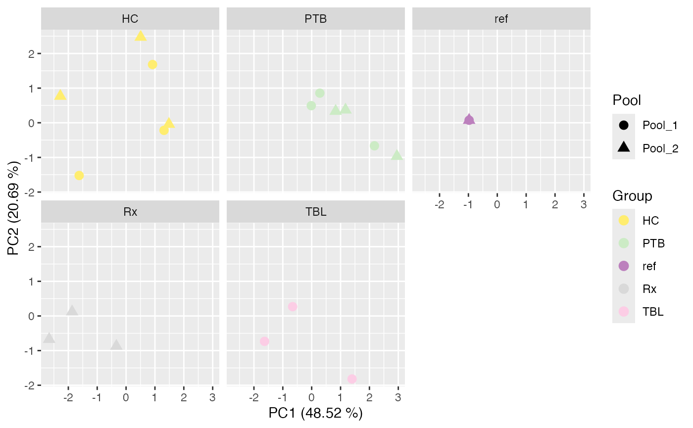
#>
#> $IRS_on_Median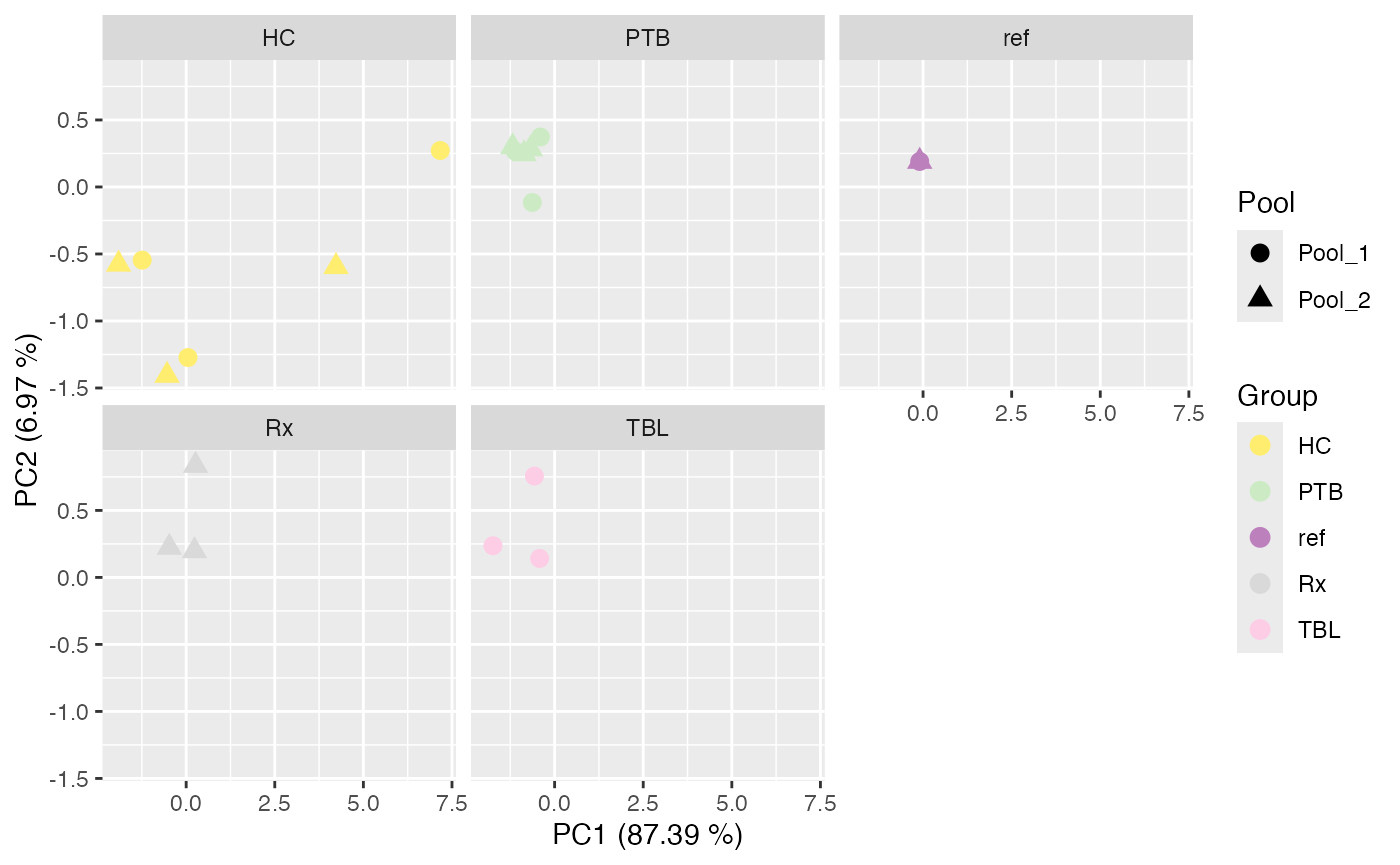
Or you can simply plot the PCA of the normalized data next to each other. However, the facet_by argument can then not be used. Reminder, by setting color_by = NULL, it will be first checked if a condition has been set in the SummarizedExperiment during loading the data.
plot_PCA(se_norm, ain = c("IRS_on_RobNorm", "IRS_on_Median"), color_by = NULL, label_by = "No", shape_by = "Pool", facet_norm = TRUE) + ggplot2::theme(legend.position = "bottom", legend.direction = "vertical")
#> Condition of SummarizedExperiment used!
#> No labeling of samples.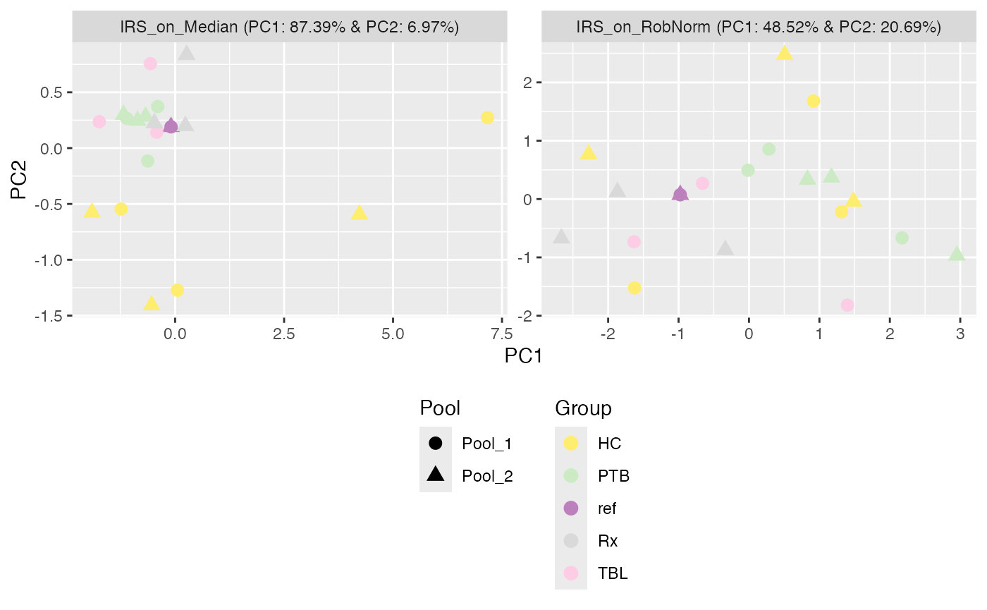
Additionally, you can add all the individual normalized sample
intensities to a big SummarizedExperiment object, and perform a single
PCA on all samples (all samples meaning samples from all normalization
methods). First, you need to create the SummarizedExperiment object
using generate_complete_SE() and then you can simply call
the plot_PCA() function.
se_complete <- generate_complete_SE(se_norm, ain = NULL) # NULL -> all assays are taken
#> All assays of the SummarizedExperiment will be used.

plot_PCA(se_complete, ain = NULL, color_by = "Normalization", label_by = "No", shape_by = "Pool", facet_norm = FALSE)
#> All assays of the SummarizedExperiment will be used.
#> No labeling of samples.
#> No faceting done.
#> $all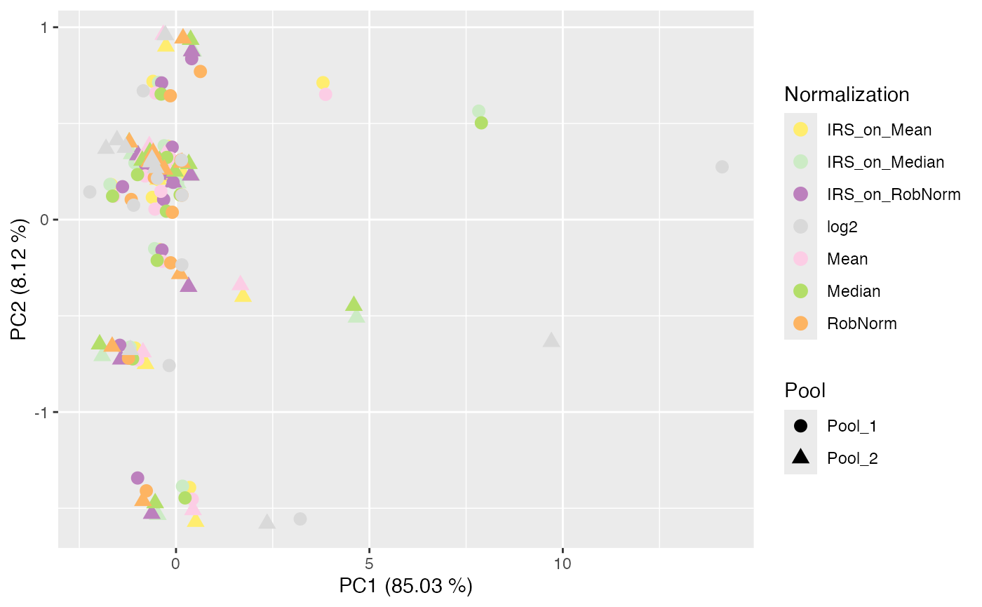
Intragroup Variation
The assessment of the normalization methods is commonly centered on their ability to decrease intragroup variation between samples, using intragroup pooled coefficient of variation (PCV), pooled estimate of variance (PEV), and pooled median absolute deviation (PMAD) as measures of variability. Furthermore, the Pearson correlation between samples is used to measure the similarity of the samples within the same group.
In PRONE, you can evaluate the intragroup variation of the normalized
data by using the functions plot_intragroup_correlation(),
plot_intragroup_PCV(), plot_intragroup_PMAD(),
and plot_intragroup_PEV().
plot_intragroup_correlation(se_norm, ain = NULL, condition = NULL, method = "pearson")
#> All assays of the SummarizedExperiment will be used.
#> Condition of SummarizedExperiment used!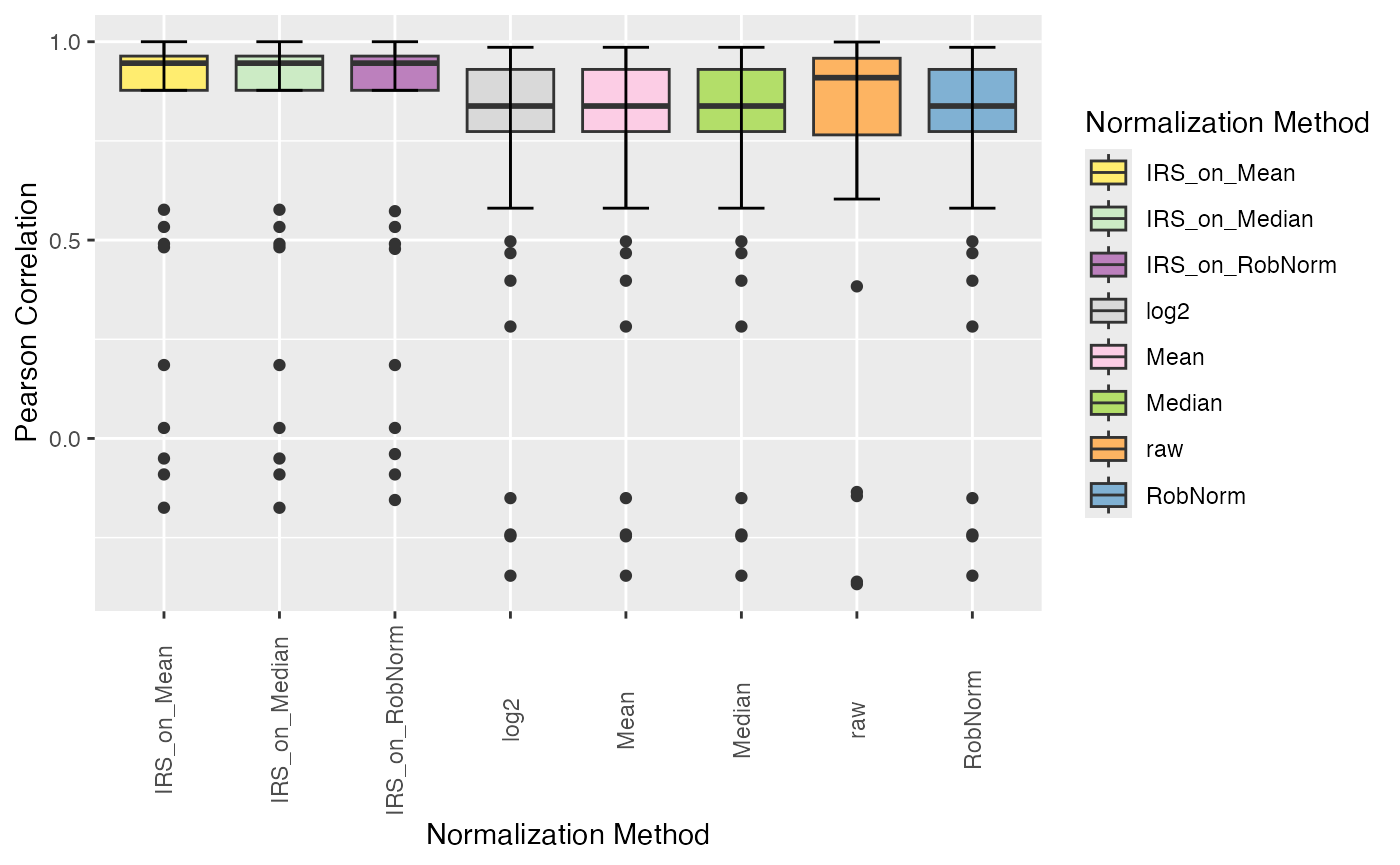
You have two options to visualize intragroup PCV, PEV, and PMAD. You can either simply generate boxplots of intragroup variation of each normalization method (diff = FALSE), or you can visualize the reduction of intragroup variation of each normalization method compared to log2 (diff = TRUE).
plot_intragroup_PCV(se_norm, ain = NULL, condition = NULL, diff = FALSE)
#> All assays of the SummarizedExperiment will be used.
#> Condition of SummarizedExperiment used!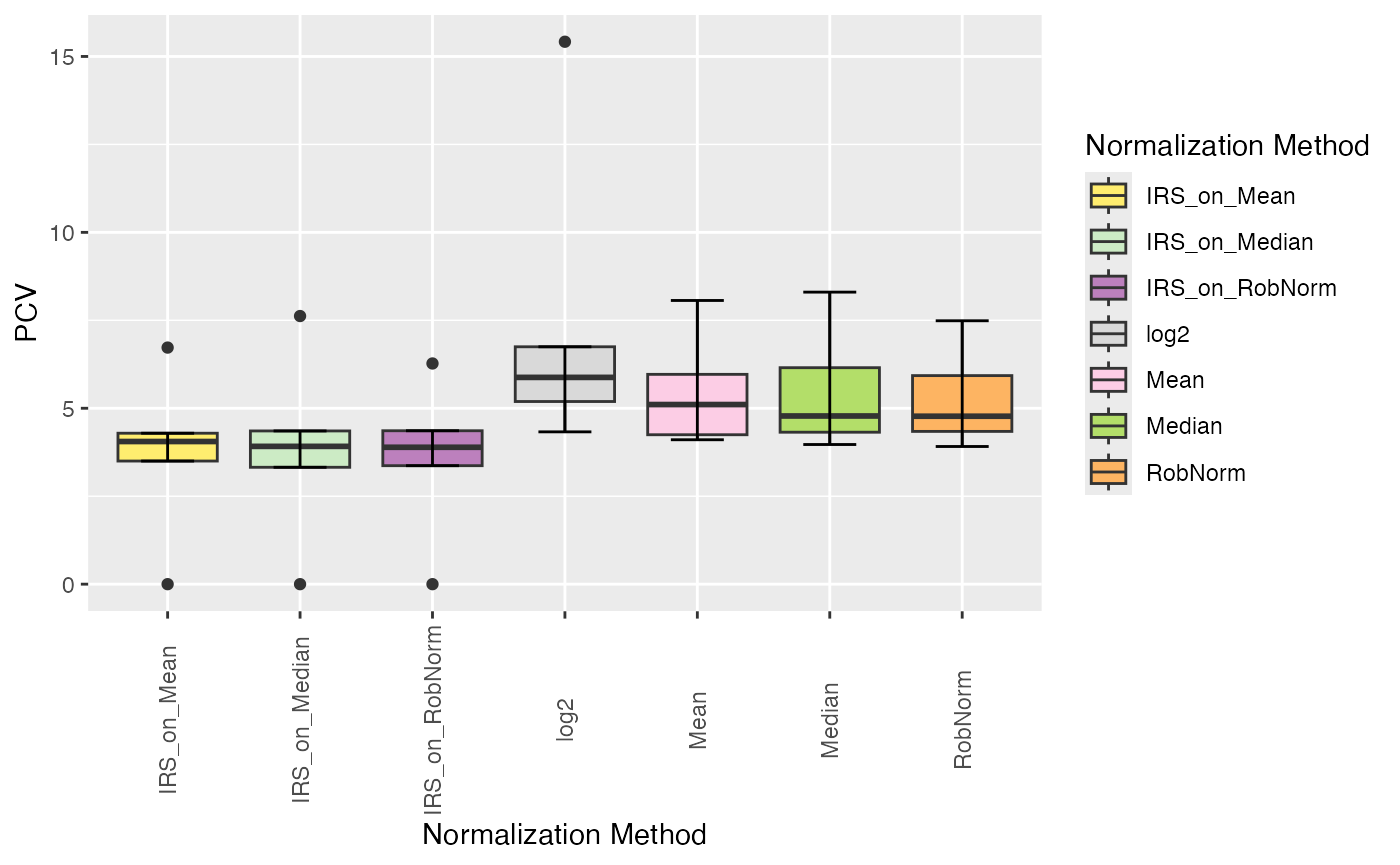
plot_intragroup_PEV(se_norm, ain = NULL, condition = NULL, diff = FALSE)
#> All assays of the SummarizedExperiment will be used.
#> Condition of SummarizedExperiment used!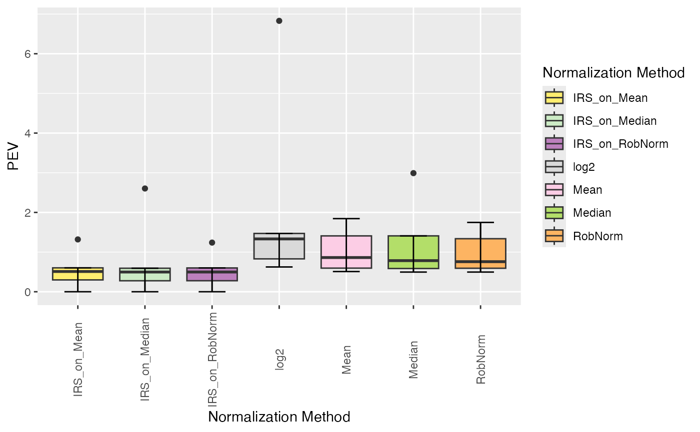
plot_intragroup_PMAD(se_norm, ain = NULL, condition = NULL, diff = FALSE)
#> All assays of the SummarizedExperiment will be used.
#> Condition of SummarizedExperiment used!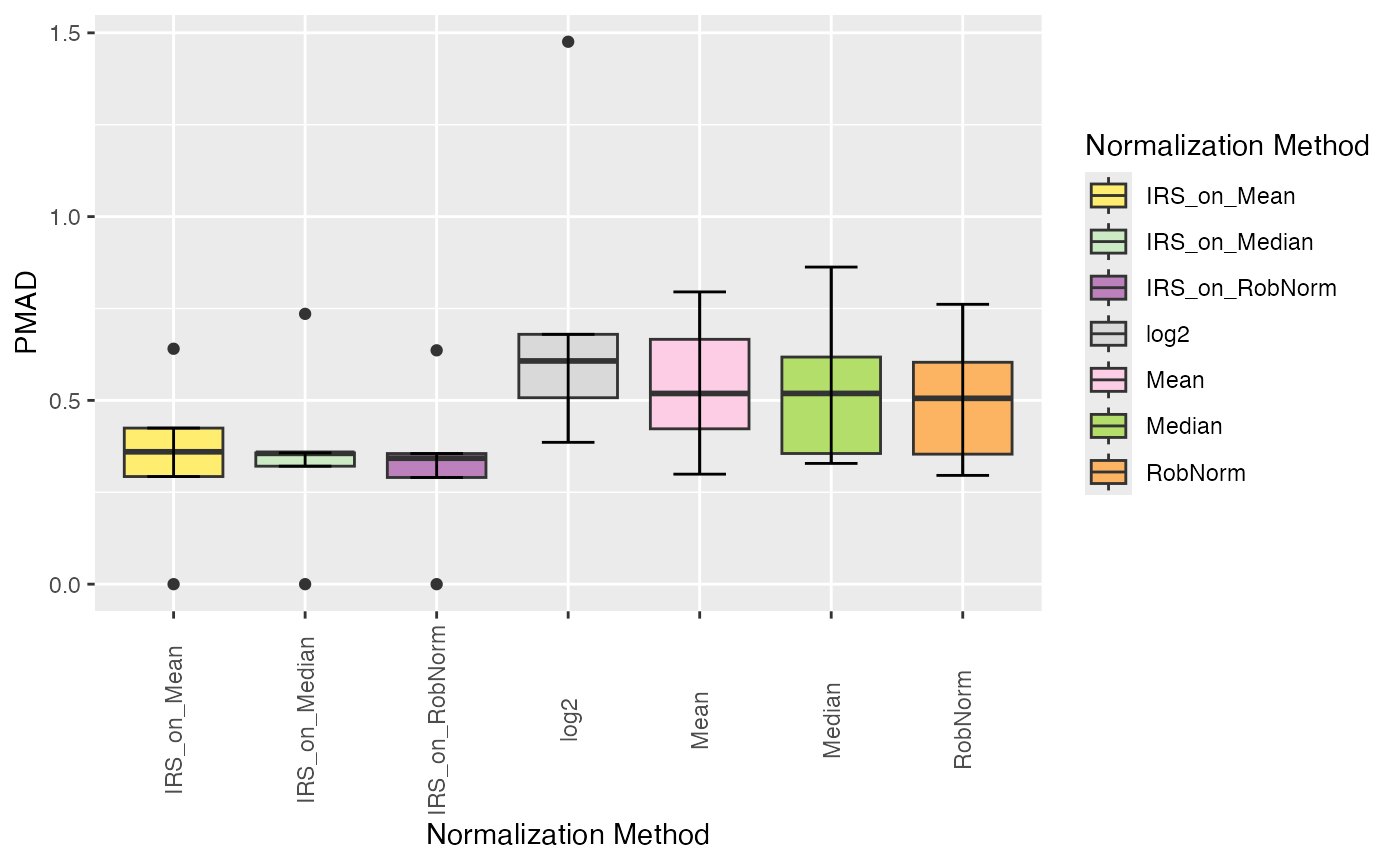
plot_intragroup_PCV(se_norm, ain = NULL, condition = NULL, diff = TRUE)
#> All assays of the SummarizedExperiment will be used.
#> Condition of SummarizedExperiment used!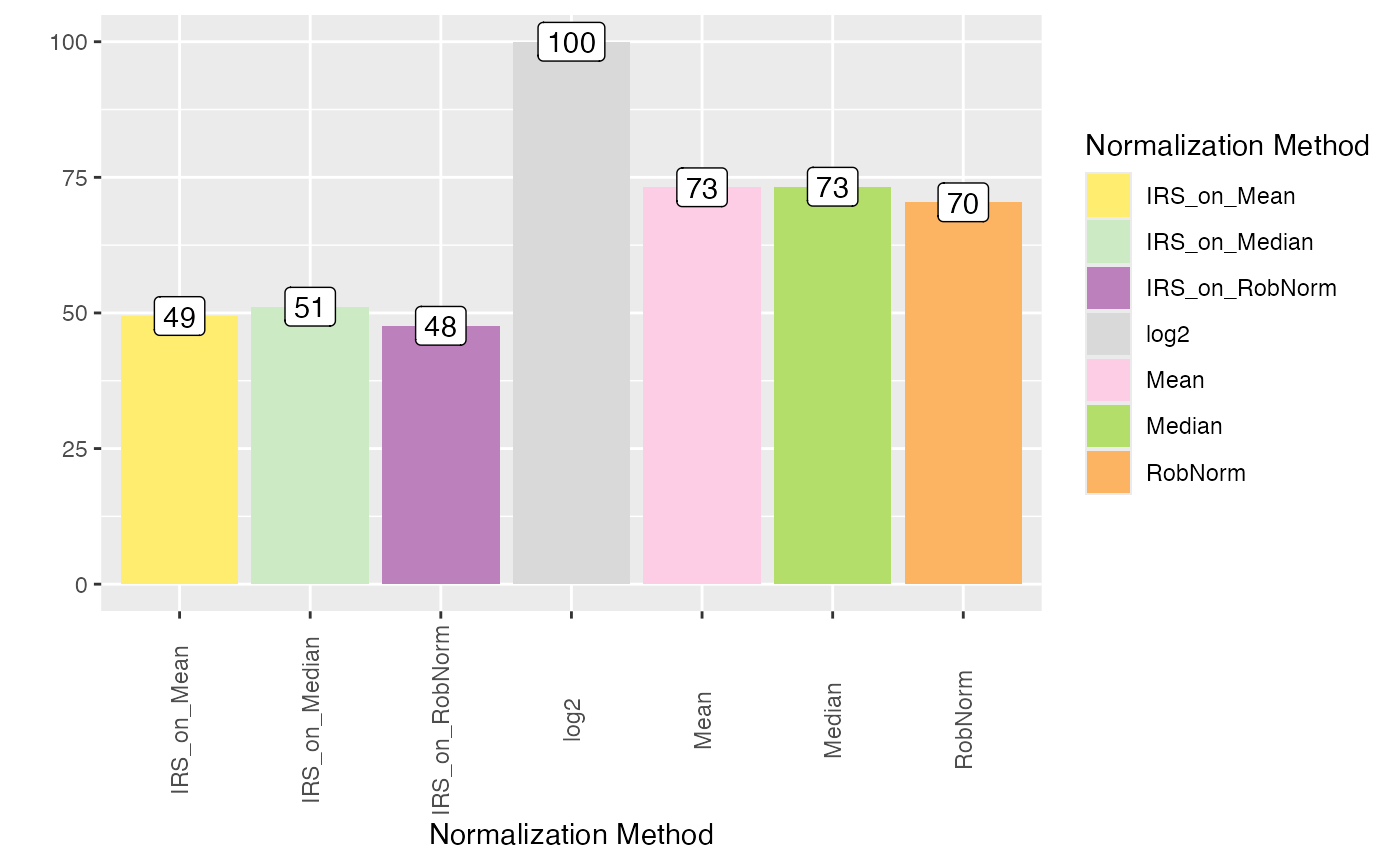
plot_intragroup_PEV(se_norm, ain = NULL, condition = NULL, diff = TRUE)
#> All assays of the SummarizedExperiment will be used.
#> Condition of SummarizedExperiment used!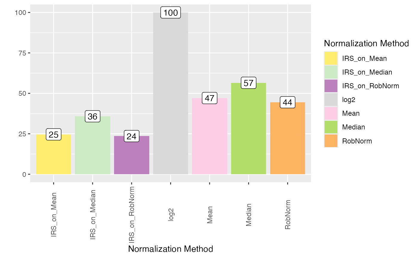
plot_intragroup_PMAD(se_norm, ain = NULL, condition = NULL, diff = TRUE)
#> All assays of the SummarizedExperiment will be used.
#> Condition of SummarizedExperiment used!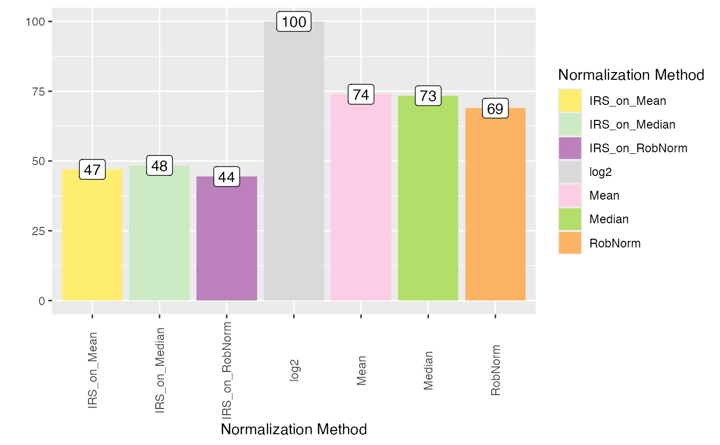
Subset SummarizedExperiment
After the qualitative and quantitative evaluation, you may have
noticed that some normalization techniques are not appropriate for the
specific real-world data set. For further analysis, you want to remove
them and not evaluate the specific normalization methods furthermore.
For this, the remove_assays_from_SE() method can be
used.
se_no_MAD <- remove_assays_from_SE(se_norm, assays_to_remove = c("MAD"))In contrast, you can also subset the SummarizedExperiment object to
only include specific normalization techniques using the
subset_SE_by_norm()method.
se_subset <- subset_SE_by_norm(se_norm, ain = c("IRS_on_RobNorm", "IRS_on_Median"))Session Info
utils::sessionInfo()
#> R version 4.4.1 (2024-06-14)
#> Platform: aarch64-apple-darwin20
#> Running under: macOS Sonoma 14.4
#>
#> Matrix products: default
#> BLAS:   /Library/Frameworks/R.framework/Versions/4.4-arm64/Resources/lib/libRblas.0.dylib
#> LAPACK: /Library/Frameworks/R.framework/Versions/4.4-arm64/Resources/lib/libRlapack.dylib;  LAPACK version 3.12.0
#>
#> locale:
#> [1] en_US.UTF-8/en_US.UTF-8/en_US.UTF-8/C/en_US.UTF-8/en_US.UTF-8
#>
#> time zone: Europe/Berlin
#> tzcode source: internal
#>
#> attached base packages:
#> [1] stats     graphics  grDevices datasets  utils     methods   base
#>
#> other attached packages:
#> [1] PRONE_0.99.6
#>
#> loaded via a namespace (and not attached):
#>   [1] rlang_1.1.4                 magrittr_2.0.3
#>   [3] clue_0.3-65                 matrixStats_1.3.0
#>   [5] compiler_4.4.1              systemfonts_1.1.0
#>   [7] vctrs_0.6.5                 reshape2_1.4.4
#>   [9] stringr_1.5.1               ProtGenerics_1.36.0
#>  [11] pkgconfig_2.0.3             crayon_1.5.3
#>  [13] fastmap_1.2.0               XVector_0.44.0
#>  [15] labeling_0.4.3              utf8_1.2.4
#>  [17] rmarkdown_2.27              UCSC.utils_1.0.0
#>  [19] preprocessCore_1.66.0       ragg_1.3.2
#>  [21] purrr_1.0.2                 xfun_0.46
#>  [23] MultiAssayExperiment_1.30.3 zlibbioc_1.50.0
#>  [25] cachem_1.1.0                GenomeInfoDb_1.40.1
#>  [27] jsonlite_1.8.8              highr_0.11
#>  [29] DelayedArray_0.30.1         BiocParallel_1.38.0
#>  [31] parallel_4.4.1              cluster_2.1.6
#>  [33] R6_2.5.1                    RColorBrewer_1.1-3
#>  [35] bslib_0.7.0                 stringi_1.8.4
#>  [37] limma_3.60.4                GenomicRanges_1.56.1
#>  [39] jquerylib_0.1.4             iterators_1.0.14
#>  [41] Rcpp_1.0.13                 SummarizedExperiment_1.34.0
#>  [43] knitr_1.48                  IRanges_2.38.1
#>  [45] Matrix_1.7-0                igraph_2.0.3
#>  [47] tidyselect_1.2.1            rstudioapi_0.16.0
#>  [49] abind_1.4-5                 yaml_2.3.10
#>  [51] ggtext_0.1.2                doParallel_1.0.17
#>  [53] codetools_0.2-20            affy_1.82.0
#>  [55] lattice_0.22-6              tibble_3.2.1
#>  [57] plyr_1.8.9                  withr_3.0.0
#>  [59] Biobase_2.64.0              evaluate_0.24.0
#>  [61] desc_1.4.3                  xml2_1.3.6
#>  [63] pillar_1.9.0                affyio_1.74.0
#>  [65] BiocManager_1.30.23         MatrixGenerics_1.16.0
#>  [67] renv_1.0.7                  foreach_1.5.2
#>  [69] stats4_4.4.1                MSnbase_2.30.1
#>  [71] MALDIquant_1.22.2           ncdf4_1.22
#>  [73] generics_0.1.3              S4Vectors_0.42.1
#>  [75] ggplot2_3.5.1               munsell_0.5.1
#>  [77] scales_1.3.0                glue_1.7.0
#>  [79] lazyeval_0.2.2              tools_4.4.1
#>  [81] data.table_1.15.4           mzID_1.42.0
#>  [83] QFeatures_1.14.2            vsn_3.72.0
#>  [85] mzR_2.38.0                  fs_1.6.4
#>  [87] XML_3.99-0.17               grid_4.4.1
#>  [89] impute_1.78.0               tidyr_1.3.1
#>  [91] MsCoreUtils_1.16.0          colorspace_2.1-0
#>  [93] GenomeInfoDbData_1.2.12     PSMatch_1.8.0
#>  [95] cli_3.6.3                   textshaping_0.4.0
#>  [97] fansi_1.0.6                 S4Arrays_1.4.1
#>  [99] dplyr_1.1.4                 AnnotationFilter_1.28.0
#> [101] pcaMethods_1.96.0           gtable_0.3.5
#> [103] sass_0.4.9                  digest_0.6.36
#> [105] BiocGenerics_0.50.0         SparseArray_1.4.8
#> [107] farver_2.1.2                htmlwidgets_1.6.4
#> [109] htmltools_0.5.8.1           pkgdown_2.1.0
#> [111] lifecycle_1.0.4             httr_1.4.7
#> [113] NormalyzerDE_1.22.0         statmod_1.5.0
#> [115] gridtext_0.1.5              MASS_7.3-61